Variable Stars: Types, Light Curves, and How to Observe

Table of Contents

• What Are Variable Stars in Observational Astronomy?
• Major Types of Variable Stars and How They Behave
• Reading and Interpreting Light Curves for Beginners
• Planning Amateur Observations of Variable Stars
• Step-by-Step Visual and Digital Photometry Workflows
• Choosing Targets: Seasonal Lists and Difficulty Levels
• From Backyard Data to Science: Submitting and Using Results
• Common Pitfalls and Expert Tips for Reliable Results
• Frequently Asked Questions
• Final Thoughts on Choosing the Right Variable Star Targets

What Are Variable Stars in Observational Astronomy?

Variable stars are stars whose brightness changes with time as observed from Earth. These variations occur for many reasons, and they span a huge range of timescales and amplitudes—from subtle, millimagnitude fluttering over minutes to dramatic multi-magnitude swings over months. For amateur and professional observers alike, variable stars provide a rich laboratory for studying stellar interiors, binary interactions, accretion physics, and the cosmic distance scale.

Broadly, astronomers categorize variability into two classes:

• Intrinsic variability: The star’s light output truly changes. Examples include pulsating stars like Cepheids or RR Lyrae, where the star expands and contracts, and eruptive/cataclysmic variables such as dwarf novae, where accretion processes brighten the system.
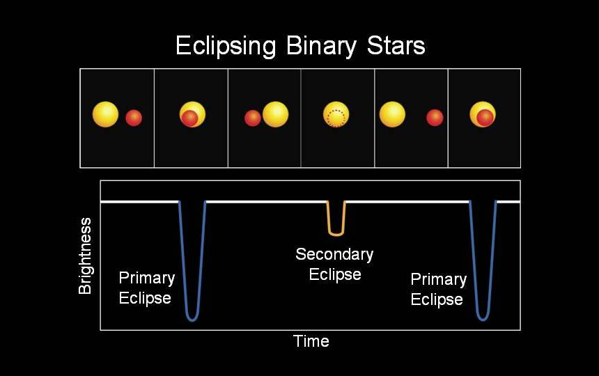
• Extrinsic variability: The star’s light doesn’t fundamentally change, but our view of it does. The classic case is an eclipsing binary where one star periodically passes in front of another, causing predictable dips in light.

Historically, variable stars have played pivotal roles in astronomy. The period–luminosity relation of Cepheids, discovered by Henrietta Swan Leavitt, underpins distance measurements to nearby galaxies and helped establish the scale of the Universe. Eclipsing binaries reveal stellar sizes and masses. Cataclysmic variables and novae illuminate disk accretion and thermonuclear processes. Today, space missions like TESS complement ground-based surveys (ASAS-SN, ZTF) and a worldwide network of amateurs coordinated through organizations such as the AAVSO (American Association of Variable Star Observers) to build continuous, long-baseline light curves.

If you’re transitioning from general stargazing or deep-sky observing, variable stars offer a compelling next step because even modest equipment can produce scientifically useful data. As you read on, you’ll see how to classify targets (types of variables), interpret their light curves (how to read light curves), plan observations (observing plans), execute photometry (workflows), and share results with the community (submitting data).

Major Types of Variable Stars and How They Behave

Knowing the chief categories of variability helps you pick targets that match your equipment and sky conditions. Below is a practical overview focused on observational behavior, timescales, and typical amplitudes.

Intrinsic pulsators

• Cepheid variables: Supergiant stars with periods of roughly 1–100 days. Their light curves are asymmetric with a rapid rise and slower decline. Amplitudes typically range from ~0.2 to 2 magnitudes. Because period correlates strongly with absolute magnitude, Cepheids are crucial standard candles in cosmology.
• RR Lyrae stars: Older, low-mass stars with short periods (~0.2–1 day). They show characteristic sawtooth or sinusoidal light curves with amplitudes ~0.3–1 mag. Their relatively uniform intrinsic brightness makes them standard candles within the Milky Way.
• Mira and long-period variables (LPVs): Cool red giants like Mira (Omicron Ceti) with large amplitudes (2–6 mag) and periods of ~100–500 days. They’re excellent for naked-eye or binocular monitoring when near maximum.
  

  

• Delta Scuti and SX Phoenicis: Short-period pulsators (tens of minutes to a few hours) with small amplitudes (millimagnitudes to a few tenths of a magnitude). They often require digital photometry and careful cadence planning.

Eruptive and cataclysmic variables

• Dwarf novae (e.g., SS Cyg): Interacting binaries with a white dwarf accreting matter from a companion via a disk. They exhibit semi-regular outbursts of a few magnitudes, lasting days to weeks, triggered by thermal-viscous instabilities in the disk.
• Classical/recurrent novae: Thermonuclear runaways on the white dwarf’s surface lead to large-amplitude brightenings (several to many magnitudes). These are rarer events; amateurs sometimes catch rises or follow the decline.
• Symbiotic stars: White dwarfs accreting from red giant winds; they can show slow changes, flickering, and episodic brightenings, rewarding long-term monitoring.

Rotational and spotted stars

• BY Draconis-type: Late-type dwarfs whose spotted surfaces rotate in and out of view, producing low-amplitude, quasi-periodic variations on timescales of days to weeks. Useful for studying stellar activity cycles and rotation.
• Ellipsoidal variables: Tidally distorted stars in close binaries vary as their non-spherical shapes present different projected areas to the observer over the orbit, typically with two maxima and two minima per cycle.

Extrinsic: eclipsing binaries and transits

• Algol-type (EA): Detached binaries with flat maxima and sharp, well-defined primary minima when one star eclipses the other. Algol (Beta Persei) is a classic: a period of ~2.867 days with a primary dip of about 1.3 mag, making it ideal for timed campaigns.
• Beta Lyrae-type (EB): Semi-detached binaries with continuously changing light owing to tidal distortion and ongoing mass transfer. The minima are rounded; Beta Lyrae’s period is ~12.9 days.
• W Ursae Majoris-type (EW): Contact binaries with short periods (0.2–0.8 days). Light curves show nearly equal minima and small amplitudes, great for high-cadence digital photometry.
• Exoplanet transits: While not a “variable star” in the traditional sense, transiting planets cause shallow, periodic dips. Detecting these typically requires millimagnitude precision and careful systematics control, but many amateur setups can capture transits of brighter hosts with well-characterized ephemerides.

As you decide on targets, think about cadence, amplitude, and observability. For fast pulsators and EW binaries, you need short exposures and precise timing. For LPVs, weekly estimates suffice and can be done visually. For more on matching targets to your setup, see Choosing Targets and the planning advice in Planning Amateur Observations.

Reading and Interpreting Light Curves for Beginners

A light curve is a plot of brightness versus time. Being able to read one quickly tells you a lot about the underlying physics, and it also helps you debug your own data. Here are the core concepts:

• Magnitude and flux: Astronomers use logarithmic magnitudes; smaller numbers mean brighter light. A 1-magnitude difference corresponds to a brightness ratio of about 2.512. Differential photometry measures your target’s brightness relative to stable comparison stars.
• Period: The time it takes for one cycle to repeat. Eclipsing binaries have orbital periods; pulsators have pulsation periods. Many analyses use phase-folded light curves, where time is mapped into phase (0 to 1) using a trial period.
• Amplitude: The peak-to-peak brightness variation. It hints at the mechanism: large amplitudes are common in LPVs and eruptive variables; small amplitudes are common in rotational variables and many exoplanet transits.
• Shape: Cepheids often show a steep rise and gradual fall; EA binaries show flat maxima with sharp minima; EW binaries are more sinusoidal and continuous; dwarf novae show outbursts with fast rise, slower decay.
  

  

Sampling and cadence

To recover a reliable period and shape, you need adequate time sampling. Undersampling produces aliasing—spurious periods introduced by gaps in your data. Daily observing windows can create strong aliases at 1 cycle/day (and harmonics). A combination of multi-longitude observers or extended nightly coverage helps break alias patterns. See the planning tips in Planning Amateur Observations for cadence guidance.

Period finding and diagnostics

• Lomb–Scargle periodogram: A widely used method for unevenly sampled data. Peaks in the periodogram suggest candidate periods; cross-check with phase plots.
• Fourier analysis: Decomposes the light curve into sinusoidal components. For pulsators with multiple modes, Fourier terms help characterize shape and harmonics.
• O–C diagrams (Observed minus Calculated): Track timing residuals of maxima or minima versus a reference ephemeris. Useful for detecting period changes, mass transfer, or light-time effects in binaries.

Color and filters

Observations in multiple passbands (e.g., Johnson–Cousins B, V, Rc, Ic or Sloan g’, r’, i’) reveal temperature changes and reddening. Cepheids, for instance, are cooler at minimum and hotter at maximum, shifting color indices (B–V). If you’re starting out, the V band is the most universally useful for comparison with published sequences and for submitting data to common databases. More on filters appears in Planning Amateur Observations and Photometry Workflows.

Planning Amateur Observations of Variable Stars

Good planning ensures that your time under the stars produces high-quality, scientifically valuable measurements. This section covers target selection, equipment, filters, exposure times, and essential calibration.

Target selection and resources

• Catalogs and alerts: The AAVSO’s Variable Star Index (VSX) provides classifications, periods, and magnitude ranges. Survey alerts (e.g., from ASAS-SN) highlight current outbursts and interesting events. Many observers plan nightly targets based on these feeds combined with seasonal visibility.
• Comparison charts: Use reliable charts with photometric sequences. The AAVSO’s chart tools provide vetted comparison stars with calibrated magnitudes in standard filters. Sticking to a documented sequence helps maintain consistency over months or years.
• Ephemerides: For eclipsing binaries and exoplanet transits, consult predicted minima or transit times. Plan to start observing well before the event and continue well after to establish a baseline.
  

  

Equipment: from naked eye to CCD/CMOS

• Visual observing: For LPVs and bright eclipsing binaries, you can contribute with just your eyes or binoculars. A small telescope (e.g., 80–150 mm) extends your reach substantially.
• Digital imaging: Affordable CMOS cameras and DSLRs enable precise differential photometry. A modest equatorial mount with tracking, a small refractor or SCT, and stable focusing are the essentials.
• Guiding and tracking: For short exposures typical of bright variables, guiding isn’t always necessary. For faint targets or long series, guiding improves SNR and keeps stars on the same pixels, reducing flat-field related systematics.

Filters and passbands

• V filter (Johnson–Cousins): The de facto standard starting point, matching a wealth of archival data. Many comparison sequences specify V magnitudes.
• B, Rc, Ic: Useful for color information and for variables where amplitude differs strongly by wavelength (e.g., cooler LPVs).
• Sloan g’, r’, i’: Increasingly common in surveys; amateurs can contribute by transforming to standard systems or by reporting in these bands where supported.
• No filter (clear): Maximizes throughput but mixes spectral response; if used, specify the camera’s response and be cautious about color-dependent systematics.

Exposure time and cadence

Choose exposures that avoid saturation while providing a healthy signal-to-noise ratio (SNR). For fast variables (e.g., EW binaries, delta Scuti), aim for a cadence of 30–120 seconds; for EAs near eclipse, you might do shorter exposures and stack if necessary. For LPVs, a single measurement every few days or weekly is fine. The Sampling and cadence notes apply: consistent spacing and adequate baseline coverage are key.

Calibration frames

• Bias frames: Zero-second exposures that measure the readout offset; some modern CMOS workflows prefer using dark flats instead of separate biases.
• Dark frames: Match your exposure time and temperature; subtracts thermal noise.
• Flat fields: Correct for vignetting and pixel-to-pixel sensitivity variations. Use twilight flats or an evenly illuminated panel; capture enough frames to build a low-noise master flat.

Keep notes on conditions, including transparency, seeing, and any filter or focus changes. Good metadata supports quality control and helps when you submit results.

Step-by-Step Visual and Digital Photometry Workflows

Whether you prefer traditional visual estimates or millimagnitude-precision digital photometry, a repeatable workflow ensures that your data are reliable and comparable with the broader community’s measurements.

Visual estimating

1. Prepare charts: Print or load a chart with labeled comparison stars and their magnitudes. Confirm you can identify the field and the variable star unambiguously.
2. Dark adaptation: Allow sufficient time for your eyes to adjust. Avoid bright screens; use red light if needed.
3. Comparison method: Use the fractional method: estimate the variable’s brightness as a fraction between two comps (e.g., “v is 40% of the way from 8.1 to 7.8, so ~7.92”). Alternatively, use step estimates in 0.1–0.2 magnitude increments.
4. Record details: Note the time (UTC), estimate, comparison stars used, sky conditions, and instrument. Aim for consistent methodology session to session.
5. Submit promptly: Visual estimates build valuable long-term light curves, especially for LPVs and bright eclipsing binaries.

Digital differential photometry

1. Acquire data: Capture a time series with stable focus and pointing. Use a filter if possible (V is a good start). Avoid saturating your target or comps.
2. Calibrate images: Apply bias/dark/flat corrections to every light frame. Ensure masters are recent and well-matched to your session.
3. Astrometric alignment: Plate solve and align frames so that apertures fall consistently on the same stars, reducing photometric scatter from pixel-level response differences.
4. Aperture photometry: In software like AstroImageJ, AIJ, Maxim DL, or AAVSO VPhot, select circular apertures for the target, one or more comparison stars, and a check star. Set an appropriate sky annulus to estimate and subtract background.
5. Differential magnitudes: Compute the variable’s magnitude relative to the comp(s). A check star confirms stability; its measured magnitude should remain constant within errors.
6. Error estimation: Report photometric uncertainties based on photon statistics, read noise, and background variance. Your software will provide per-point errors; ensure they are realistic (neither underestimated nor overly conservative).
7. Transformations: If you intend to combine data with observations from other systems, consider deriving transformation coefficients to place your results onto the standard system (e.g., Johnson–Cousins V). This corrects for color terms in your instrument’s spectral response.

Many observers also use differential extinction corrections if the target and comps differ in altitude or color, especially at high airmass. Keeping target and comp stars close in the sky and color reduces this need.

Software tools and file hygiene

• AstroImageJ (AIJ): Popular, free tool for time-series photometry, including exoplanet transits and variable stars.
• AAVSO VPhot: Web-based photometry for members; integrates with AAVSO charts and comp sequences.
• Peranso, Period04: Period search and light-curve analysis tools; support Lomb–Scargle, Fourier methods, and more.

Adopt consistent file naming and metadata practices. For example:

2026-08-17_Algol_V_60s_series.fit
# Include FITS headers: OBJECT=Algol, FILTER=V, EXPTIME=60, JD, AIRMASS, OBSERVER

For visual and digital observations alike, correlating your raw data with processed results and logs helps track down issues later. This becomes essential as you join campaigns described in From Backyard Data to Science.

Choosing Targets: Seasonal Lists and Difficulty Levels

Here are widely observed, well-characterized targets that accommodate different skill levels and equipment. Magnitude ranges and periods are typical values; consult current databases for up-to-date ephemerides and states. If your latitude differs significantly from mid-northern or mid-southern, adjust seasonal timing accordingly.

Beginner-friendly, bright variables

• Algol (Beta Persei): EA eclipsing binary; P ≈ 2.867 days; primary eclipse depth ~1.3 mag. Easy to estimate visually during predicted minima; valuable timing target.
• Delta Cephei: Prototype Cepheid; P ≈ 5.366 days; amplitude ~0.7 mag in V. Great for learning to phase-fold and appreciate the period–luminosity relation.
• Mira (Omicron Ceti): LPV; P ≈ 332 days; range ~2–10 mag. A classic naked-eye variable at maximum, rewarding long-term visual monitoring.
• Beta Lyrae: EB-type eclipsing binary; P ≈ 12.9 days; smooth, continuous variation requires nightly series for shape.
• RR Lyrae (various field stars): P ≈ 0.2–1 day; amplitude ~0.3–1 mag. Choose a bright field RR Lyrae suitable for your setup to practice short-period photometry.

Intermediate: small amplitudes and higher cadence

• W Ursae Majoris systems (e.g., 44 Boo): EW contact binaries; P ≈ 0.2–0.8 days; amplitude often < 0.8 mag. Ideal for honing cadence and precision.
• Delta Scuti stars: Multi-mode pulsators with periods of 0.02–0.3 days; low amplitude demands consistent photometric technique and error control.
• SS Cygni: Dwarf nova with outbursts every several weeks; amplitude ~2–3 mag. Follow alert networks to catch rises and document decays.

Advanced: faint or challenging systematics

• Semi-regular red giants: Amplitudes and periods vary; combining long-term visual with filtered photometry reveals complex behavior.
• Eclipsing binaries with shallow minima: Good for exploring millimagnitude precision and systematics control, especially under bright skies.
• Exoplanet transits of bright hosts: Depths of a few to tens of millimagnitudes. Demands careful differential photometry, stable focus/pointing, and robust detrending.

Seasonal visibility considerations

Plan targets that culminate high in the sky to minimize airmass and extinction. For northern mid-latitudes, winter offers Betelgeuse (a semiregular red supergiant with notable variability episodes), while autumn favors Algol at convenient evening hours. Southern observers might emphasize bright LPVs like R Carinae in appropriate seasons. When in doubt, consult a planetarium app to visualize altitude and transit times, then build a list that balances quick targets and long-term projects. Cross-reference your choices with planning tips and with the submission requirements to ensure your data match community standards.

From Backyard Data to Science: Submitting and Using Results

One of the most rewarding aspects of variable star observing is that your data can contribute directly to research. Organizations coordinate observations, curate extensive databases, and make data discoverable for analysis. Here’s how to go from raw measurements to community contributions.

Choose a destination for your data

• AAVSO: A widely used repository for visual and digital variable star data. Its tools and documentation guide you through choosing comparison stars, formatting reports, and interpreting quality metrics.
• Campaigns and alerts: Collaborative efforts request specific timing and filters for targets experiencing interesting states (e.g., outbursts, eclipses, or long-term period changes). Coordinated multi-longitude efforts reduce aliasing and fill in light curves.

Time standards and timestamps

Accurate timekeeping is essential, especially for short-period variables. Synchronize your acquisition computer’s clock with a reliable time source before observing. Many observers convert timestamps to Julian Date (JD) in UTC for reporting, and some workflows use Heliocentric Julian Date (HJD) or Barycentric Julian Date (BJD) to correct for Earth’s motion—this matters for precise timing analyses. Follow your destination’s guidelines on which time standard to report; ensure clarity in metadata.

Formatting observations

When submitting, you’ll typically include target ID, time (JD/HJD/BJD as specified), magnitude, uncertainty, filter, comparison stars, and equipment notes. A simple CSV row might look like:

Target,JD,Mag,Err,Filter,Comp,Check,Observer,Notes
Algol,2460253.7431,3.58,0.01,V,HD 19356,HD 19400,YourCode,\"Primary eclipse in progress\"

Be consistent in your comparison star selection and document any changes across nights. If your comp star saturates or drifts into a vignetted region, switch to a documented alternative and note it clearly.

Quality control

• Reject poor frames: Remove images with trailed stars, clouds, or guiding loss. Inspect the background for gradients.
• Check star stability: The check star residuals should scatter around a constant value within reported errors; large deviations hint at systematics.
• Photometric flags: Use flags to indicate partial clouds, high airmass, or focus changes. Transparency fluctuations can mimic astrophysical variations if unflagged.

Clean, well-documented light curves are easier for others to combine with different datasets, including survey data. For additional context, see Interpreting Light Curves and Common Pitfalls.

Common Pitfalls and Expert Tips for Reliable Results

Even experienced observers encounter systematic errors. Recognizing and mitigating them elevates your results from good to excellent.

Systematics to watch

• Saturation and nonlinearity: Avoid pushing stars near your camera’s full-well capacity. Nonlinear response distorts magnitudes. Shorten exposures or defocus if needed.
• Flat-field errors: Dust motes and vignetting can introduce false variability. Update flats when you rotate the camera or change the optical path.
• Color mismatch: If your target is very red and comps are blue (or vice versa), differential extinction and untransformed passbands will bias results. Use comps with similar color or apply transformations.
• Crowding and blending: In dense fields, overlapping PSFs can contaminate apertures. Smaller apertures with careful sky annuli, or PSF photometry, may be necessary.
• Transparency fluctuations: Passing clouds cause correlated dips and rises. A stable check star reveals this; if both target and check dip, it’s likely weather, not astrophysics.
• Timing drift: Unsynced clocks smear phase plots for short-period targets. Regularly sync time to avoid accumulating errors.

Techniques that help

• Defocus strategically: Spreading starlight over more pixels avoids saturation and reduces intrapixel sensitivity effects, improving precision for bright stars.
• Maintain constant focus and pointing: Consistency minimizes flat-field and seeing-induced variations. If you must refocus, note the change and recheck aperture sizes.
• Use multiple comps: An ensemble of comparison stars often provides better stability than a single comp. Ensure they’re of similar color and not variable.
• Monitor airmass: Observing near the meridian reduces extinction. If high airmass is unavoidable, keep target and comps at similar altitudes.
• Report realistic errors: Underestimated errors give a false impression of precision; overestimated ones dilute your contribution. Calibrate your pipeline with stable stars.

Analysis enhancements

• Detrending: Remove slow trends from changing airmass or temperature using comparison ensembles or decorrelation against parameters (e.g., sky background, FWHM).
• Period refinement: Combine your data with archival measurements and survey light curves to refine periods and ephemerides. An updated O–C diagram can reveal period changes or additional bodies.
• Cross-validation: Compare your measurements with those from observers using different equipment or bands to identify persistent discrepancies.

Build these checks into your routine, and your datasets will integrate more cleanly with community archives. When in doubt, revisit the foundations in Planning and Workflows.

Frequently Asked Questions

Can I do useful variable star observing from a light-polluted city?

Yes. While light pollution affects faint deep-sky objects, many variable star projects remain viable in bright skies. Visual estimates of brighter LPVs and eclipsing binaries are practical from urban locations. For digital work, differential photometry cancels much of the skyglow’s impact: as long as your target and comps are well measured within each frame, you can achieve high precision. Use shorter exposures to avoid saturating the sky background, choose targets high above the horizon, and employ filters (V or r’) to stabilize your bandpass. Conduct careful calibration and keep stars on the same pixels; stacking short exposures can help for faint targets. For short-period variables or exoplanet transits, urban observers often achieve millimagnitude precision with attention to detrending and systematics.

What filter should I buy first for photometry?

If you’re buying just one, choose a Johnson–Cousins V filter. It’s the most commonly used in amateur–professional collaborations and matches a vast archive of comparison star magnitudes. Adding Rc or Ic next expands your reach to redder variables like LPVs and cool eclipsing binaries. If your projects align with modern survey data in Sloan bands, a g’ or r’ filter is also valuable. Whichever you pick, document your passband and, if possible, derive transformation coefficients so your data inter-compare reliably with others.

Final Thoughts on Choosing the Right Variable Star Targets

Variable stars offer a uniquely satisfying blend of accessibility and scientific impact. With little more than a reliable mount, a small telescope or binoculars, a thoughtful observing plan, and attention to calibration, you can produce data that matter. Start with forgiving, bright targets like Algol, Delta Cephei, and Mira to learn cadence, visual estimating, and basic photometry. As your proficiency grows, explore short-period EW binaries, delta Scuti pulsators, and cataclysmic variables. Apply the best practices outlined in planning, workflows, and pitfalls to improve reliability, and share your results through community databases. The night sky is dynamic, and your measurements help reveal its rhythms—cycle by cycle, season by season.

If you found this guide useful, consider subscribing to our newsletter for upcoming deep-dives into specific variable classes, tutorials on period analysis, and seasonal target lists. We regularly publish practical observing guides and science explainers to help you expand your capabilities and contribute to ongoing research.