Pulsar Timing Arrays and the Hum of Spacetime

Table of Contents

• What Is Pulsar Timing and Why It Matters
• How Millisecond Pulsars Work: Cosmic Clocks in Practice
• Building a Pulsar Timing Model: From Observatory to Barycenter
• Pulsar Timing Arrays and the Nanohertz Gravitational-Wave Background
• Noise, Systematics, and How We Mitigate Them
• From Pulses to Physics: Data Analysis and Inference
• Key Science Results: Gravity, Galaxies, and the Interstellar Medium
• Receivers, Backends, and Calibration: The Hardware Behind Timing
• How to Get Involved: Software, Data, and Citizen Science
• Frequently Asked Questions
• Final Thoughts on Pulsar Timing Arrays and Cosmic Clocks

What Is Pulsar Timing and Why It Matters

Pulsar timing is the art and science of predicting and measuring the exact arrival times of pulses from rapidly rotating neutron stars. Millisecond pulsars—old neutron stars spun-up in binary systems—are extraordinarily stable rotators, with pulse arrival times that can be forecast to microsecond precision or better. By comparing the observed times of arrival (TOAs) with the predicted times implied by a physical model, astronomers extract tiny timing residuals that contain a wealth of astrophysical information.

Why does this matter? Because any process that perturbs the path of the radio pulses or the clock used to time them can imprint a signature in those residuals. That includes:

• The rotation and orbital motion of the pulsar itself;
• Dispersive delays in the ionized interstellar medium;
• Errors in our Solar System ephemeris and terrestrial time standards;
• And, crucially, spacetime ripples—gravitational waves—passing between Earth and the pulsar.

By timing an array of pulsars spread across the sky, we obtain a long-baseline, galaxy-scale interferometer that is sensitive to gravitational waves with periods of years to decades. This is the domain of the nanohertz gravitational-wave background, thought to be generated primarily by inspiraling supermassive black hole binaries residing in the hearts of merging galaxies.

If you are familiar with laser interferometers like LIGO and Virgo, you can think of pulsar timing arrays (PTAs) as their low-frequency complement. Instead of kilometer-scale lasers responding to millisecond-scale strains, PTAs use light-years-long baselines encoded in pulsar-to-Earth light travel times to probe incredibly slow gravitational undulations. We unpack that comparison further in Frequently Asked Questions.

How Millisecond Pulsars Work: Cosmic Clocks in Practice

Pulsars are rapidly rotating neutron stars—a city-sized object with a mass around that of the Sun—whose intense magnetic fields channel charged particles into beams of radiation. As the star spins, the beam sweeps across space like a lighthouse. When it crosses our line of sight, we observe a pulse.

Millisecond pulsars (MSPs) are a special subclass with rotation periods of roughly 1–10 milliseconds. They are thought to be “recycled”: originally formed in a supernova, then spun up through accretion of matter from a companion star. This history leaves them with:

• Rapid, highly stable rotation (fractional stability rivaling atomic clocks over some timescales);
• Weaker magnetic fields than young pulsars, reducing timing noise;
• Often binary companions, enabling exquisite tests of gravity via orbital dynamics.

When we observe an MSP with a radio telescope, we detect a sequence of pulses with a stable average shape, called the pulse profile. While single pulses fluctuate, averaging many periods yields a high signal-to-noise profile that serves as a template. Cross-correlating this template with the observed data provides a precise TOA for that observation.

The precision of a TOA depends on several factors:

• Bandwidth and sensitivity: Wider bandwidth receivers and larger telescopes reduce radiometer noise.
• Observing frequency: Higher frequencies suffer less dispersion and scattering by the interstellar medium (ISM), but pulsars are fainter there; wideband approaches balance these effects.
• Integration time: Longer integrations average out stochastic pulse-to-pulse variability, improving TOA precision.
• Polarization calibration: Properly calibrated polarization prevents profile distortions that bias TOAs.

MSPs are also affected by interstellar propagation. The key effect is dispersion: lower-frequency radio waves travel more slowly through ionized plasma. This introduces a frequency-dependent delay proportional to the dispersion measure (DM), the integrated electron density along the line of sight. If DM varies with time—due to ISM turbulence or solar wind—the pulse arrival time drifts. Modeling and correcting DM is essential, a topic we return to in Noise, Systematics, and How We Mitigate Them.

Building a Pulsar Timing Model: From Observatory to Barycenter

A pulsar timing model is a comprehensive, relativistic prediction for pulse arrival times. It accounts for the pulsar’s rotation, motion, environment, and our own observational frame. Conceptually, you can think of a timing model as a function that maps pulse number to arrival time at the detector, often written schematically as:

t_model = t_emission + Δ_Roemer + Δ_Shapiro + Δ_Einstein + Δ_Dispersion + …

Here are the essential ingredients:

• Spin parameters: The pulsar’s rotation frequency ν (or period P) and its derivative(s), characterizing spin-down due to electromagnetic braking and other torques.
• Astrometry: Right ascension, declination, proper motion, and parallax. These determine the changing light travel time as Earth orbits the Sun and moves relative to the pulsar.
• Binary motion (if present): Keplerian parameters (orbital period, eccentricity, projected semi-major axis, time of periastron) and, for relativistic binaries, post-Keplerian parameters (periastron advance, gravitational redshift/time dilation, Shapiro delay terms).
• Propagation: Dispersion measure and, in wideband models, frequency-dependent profile evolution and scattering.
• Reference frames and time standards: Conversion from observatory time to a uniform terrestrial timescale and then to a Solar System barycentric coordinate time, incorporating relativistic corrections.

Several corrections are central:

• Roemer delay: The geometric light travel time from Earth to the Solar System barycenter (SSB). This depends on Earth’s position, obtained from high-precision planetary ephemerides.
• Einstein delay: Time dilation and gravitational redshift due to Earth’s motion and the Sun’s gravitational potential.
• Shapiro delay: Additional time delay as pulses pass through curved spacetime near massive bodies, measurable both in binary pulsar systems and when the line of sight passes near Solar System planets or the Sun.
• Dispersion delay: Frequency-dependent plasma delay proportional to DM × ν^{-2}.

Timing packages such as TEMPO, TEMPO2, and PINT implement these models. Observations begin with TOAs stamped against a stable local clock, synced to international standards. They are then converted to a uniform terrestrial timescale (such as TT) and finally to a barycentric coordinate time using a planetary ephemeris. Commonly used ephemerides include modern releases from JPL that tabulate planetary and lunar positions with high precision for this purpose.

After fitting the model to the data, we examine the residuals:

R(t) = t_observed − t_model

Ideally, residuals are white (uncorrelated) and Gaussian-distributed around zero. In practice, they exhibit a combination of white noise and temporally correlated red noise from astrophysical, instrumental, and environmental sources. The correlations across different pulsars are the key to detecting a stochastic gravitational-wave background, as discussed in Pulsar Timing Arrays and the Nanohertz Gravitational-Wave Background.

Pulsar Timing Arrays and the Nanohertz Gravitational-Wave Background

A pulsar timing array (PTA) is a set of precisely timed MSPs distributed across the sky. By observing many pulsars over long time spans (years to decades), PTAs search for a common signal imprinted by gravitational waves (GWs). In the nanohertz band, the leading predicted source is the stochastic superposition of many inspiraling supermassive black hole binaries (SMBHBs). Other possible contributors include relic signals from the early Universe, such as cosmic strings or phase transitions, though current evidence is most consistent with SMBHBs.

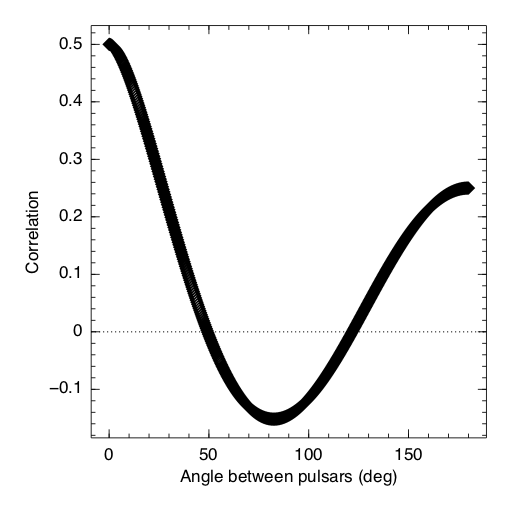
What does a gravitational-wave background do to pulsar timing? A passing GW perturbs spacetime, altering the effective light travel time between the pulsar and Earth. Each pulsar’s residuals thus contain two contributions: the “pulsar term” imprinted near the pulsar long ago, and the “Earth term” imprinted when the wave passes near Earth. The pulsar terms are uncorrelated among different pulsars, but the Earth terms are shared and produce a characteristic spatial correlation pattern between pairs of pulsars.

For an isotropic, stochastic background in general relativity, this correlation is the celebrated Hellings–Downs curve: a specific quadrupolar function of the angular separation between pulsar pairs. Detecting this pattern is the smoking gun for a nanohertz GW background. PTA collaborations have reported evidence consistent with such spatial correlations, strengthening the case for a common-spectrum process of gravitational origin in millisecond pulsar timing data.

Several international collaborations operate PTAs, often combining results into a global effort:

• North American Nanohertz Observatory for Gravitational Waves (NANOGrav)
• European Pulsar Timing Array (EPTA)
• PARKES Pulsar Timing Array (PPTA)
• Indian Pulsar Timing Array (InPTA)
• Chinese Pulsar Timing Array (CPTA)
• International Pulsar Timing Array (IPTA) for combined analyses

PTAs are sensitive to GW frequencies of order one cycle per observational timespan—roughly nanohertz frequencies corresponding to periods of years. The expected characteristic strain from SMBHBs in this band is small (amplitudes typically quoted around the order of 10⁻¹⁵ at a reference frequency of one cycle per year), but detectable given sufficient timing precision, number of pulsars, and duration.

One of the appealing aspects of PTAs is synergy with other observatories. Galaxy surveys and time-domain astronomy aim to identify individual, bright SMBHB candidates. Space-based interferometers planned for the coming decades target milli-Hz frequencies, potentially bridging the gap between the PTA band and higher-frequency interferometers. Multi-messenger connections may eventually enable
identification of individual binaries in the nanohertz band as they slowly evolve, complementing the stochastic background evidence.

Want to understand how PTA sensitivity improves? It scales with:

• Number of pulsars in the array;
• Timing precision of each pulsar (lower TOA uncertainty is better);
• Cadence (how often you observe each pulsar);
• Total timespan of the dataset (long baselines probe lower frequencies and sharpen sensitivity).

These levers motivate ongoing improvements in both instrumentation and observing strategies, as detailed in Receivers, Backends, and Calibration.

Noise, Systematics, and How We Mitigate Them

Extracting nanosecond to microsecond signals from years of data means contending with a zoo of noise sources. Understanding and mitigating them is a central part of PTA science. Key contributors include:

• Radiometer noise: Thermal noise from the receiver and sky. Improves with bandwidth and telescope sensitivity.
• Pulse phase jitter: Intrinsic variability in single pulses, which averages down with longer integrations but sets a floor for very bright pulsars.
• Dispersion measure (DM) variations: Changes in the ISM and solar wind electron content introduce chromatic (frequency-dependent) delays. Wideband timing and multi-frequency observations model and remove these.
• Scattering and profile evolution: Multi-path propagation broadens pulses, and intrinsic profile shapes vary with frequency. Wideband profile modeling jointly fits TOAs and DM to avoid bias.
• Clock errors: Deviations in terrestrial time standards introduce a monopolar correlated signal across all pulsars.
• Solar System ephemeris errors: Uncertainties in planetary masses and positions generate a dipolar correlated signal across the sky.
• Instrumentation systematics: Backend changes, polarization miscalibration, and radio-frequency interference (RFI) can imprint spurious trends.

To address these, PTA pipelines employ a combination of observational strategy and statistical modeling:

• Multi-frequency cadence: Observe each pulsar at two or more well-separated frequencies to solve for time-varying DM and disentangle chromatic from achromatic delays.
• Wideband timing: Fit the entire frequency-dependent profile simultaneously, allowing for profile evolution, DM, and TOA to be constrained in a unified model.
• Polarization calibration: Use well-understood calibrators and noise diodes to correct instrumental polarization, stabilizing profile shapes.
• Backend consistency: Overlap observations during hardware transitions and include jump parameters for inter-backend offsets.
• Ephemeris and clock modeling: Include nuisance terms for global clock deviations and ephemeris perturbations; test against multiple planetary ephemerides.
• RFI excision: Identify and remove corrupted frequency channels or time ranges; use robust statistics to limit outlier impact.

Because different noise sources have distinct spatial correlation signatures—monopolar for clocks, dipolar for ephemerides, quadrupolar for GWs—joint modeling across the array helps separate them. The ability to distinguish these correlations is what makes PTAs so powerful, and is a central theme of From Pulses to Physics: Data Analysis and Inference.

From Pulses to Physics: Data Analysis and Inference

Turning residuals into discoveries relies on careful statistical methods. At a high level, PTA analysis aims to fit both deterministic timing models for each pulsar and stochastic processes shared across the array. Two complementary approaches are common:

• Frequentist cross-correlation searches: Compute pairwise cross-correlations of residuals and compare to the expected Hellings–Downs curve.
• Bayesian inference: Simultaneously fit stochastic processes—such as a power-law gravitational-wave background—and noise parameters across the array, obtaining posterior distributions and model evidences.

A typical Bayesian model might include:

• White noise parameters per pulsar (e.g., EFAC and EQUAD terms to scale and add to TOA errors);
• Red noise per pulsar, modeled as a Gaussian process with a power-law spectrum;
• A common-spectrum process across all pulsars, optionally with Hellings–Downs spatial correlations;
• Global clock and ephemeris perturbation processes with distinct spatial templates;
• Time-varying DM as a separate, chromatic Gaussian process.

Model selection uses evidence ratios (Bayes factors) to assess whether data prefer a pure red noise model, a common-spectrum process without spatial correlations, or a fully spatially correlated Hellings–Downs signal. Priors, hyperparameters, and different parametrizations (e.g., in terms of characteristic strain amplitude and spectral index) are explored to test robustness.

For clarity of notation, one common parametrization for a stochastic background uses a power-law characteristic strain spectrum:

h_c(f) = A (f / f_ref)^{α}

For a population of circular, gravitational-wave-driven SMBHBs, the spectral index is expected to be α = −2/3, implying a steep red spectrum. Deviations from this could indicate environmental effects (e.g., interactions with stars or gas that stall or accelerate binary evolution) or alternative sources such as cosmic strings.

Key idea: PTAs fit the timing model and the noise model together. The gravitational-wave signal is inferred not as a sharp “line” but as a correlated red process spanning years of data.

Since data spans now reach up to decades for some pulsars, analyses must also contend with non-stationarities, uneven cadences, and evolving instrumentation. Techniques such as Gaussian-process modeling, time-domain likelihoods, spectral methods, and hierarchical population analyses are all employed to wring out the most information from the available data.

Key Science Results: Gravity, Galaxies, and the Interstellar Medium

Pulsar timing science extends well beyond the GW background detection. Here are the major pillars of discovery and measurement enabled by MSPs and PTAs:

Evidence for a Nanohertz Gravitational-Wave Background

Multiple PTA collaborations have reported strong evidence for a common-spectrum, red-noise process exhibiting the spatial correlations expected from a gravitational-wave background. The inferred amplitudes are consistent with expectations from populations of SMBHBs assembled through galaxy mergers, with characteristic strains around the order of 10⁻¹⁵ at a reference frequency of one cycle per year. While refining the spectrum and pinning down the astrophysical origins are ongoing, the observation of Hellings–Downs-like correlations represents a milestone for low-frequency gravitational-wave astronomy.

Implications include:

• Constraints on the demographics of SMBHBs: merger rates, typical masses, and orbital eccentricities.
• Clues to binary evolution physics: whether interactions with stars and gas accelerate or stall inspirals.
• Prospects for resolving individual, bright binaries as datasets grow longer and more sensitive.

We revisit future prospects in Final Thoughts on Pulsar Timing Arrays and Cosmic Clocks.

Precision Tests of General Relativity with Binary Pulsars

Binary pulsars offer classic laboratories for relativistic gravity. Timing relativistic effects—like periastron advance, gravitational redshift, and Shapiro delay—tests the strong-field regime of general relativity (GR). Several famous systems have provided stringent confirmations of GR, including measurements of orbital decay consistent with energy loss to gravitational radiation. These tests are complementary to PTA background measurements: the former probe strong-field, high-curvature dynamics in individual systems; the latter test the stochastic imprint of many distant binaries on spacetime over cosmic volumes.

Pulsar Timing as a Time Standard

An ensemble of millisecond pulsars can define a “pulsar timescale,” a clock derived from astrophysical rotators rather than atomic transitions. By averaging over many pulsars, one can suppress individual noise and search for deviations from terrestrial time standards. This provides an independent cross-check of long-term stability in timekeeping, probing timescales of years to decades.

Astrometry and the Solar System

High-precision timing yields parallaxes and proper motions for pulsars, contributing to Galactic kinematics and distance measurements. PTAs also probe the Solar System, constraining planetary masses and testing our ephemerides. Any systematic error in the SSB location would leave a dipolar signature across the array’s residuals; fitting for these has improved mass estimates for outer planets and their systems in some analyses.

Interstellar Medium Physics

DM variations, scattering, and scintillation provide a rich probe of the ionized ISM. PTAs monitor these effects over long baselines and at multiple frequencies, enabling measurements of turbulence, spatial inhomogeneities, and solar wind structure. The ability to disentangle chromatic ISM delays from achromatic signals is central to achieving PTA sensitivity and enhances our understanding of Galactic plasma physics.

Receivers, Backends, and Calibration: The Hardware Behind Timing

Sub-microsecond timing demands stable hardware and careful calibration. Key elements include:

• Wideband receivers: Modern systems cover hundreds of MHz to a few GHz of bandwidth in a single observation, boosting sensitivity and enabling wideband timing that jointly fits DM and profile evolution.
• Coherent dedispersion: Real-time or offline removal of ISM dispersion by convolving the data with the inverse transfer function of the dispersion kernel, preserving sharp pulse structure across the band.
• Digital backends: High-speed digitizers and field-programmable gate arrays (FPGAs) or GPUs to channelize, dedisperse, and fold the data, producing integrated profiles with precise timestamps.
• Stable time references: Hydrogen masers and GPS-disciplined oscillators provide the observatory’s local clock, which is tied to international standards.
• Polarization calibration: Noise diodes and polarized calibrators allow the full-Stokes response of the telescope to be measured and corrected, stabilizing the pulse profile.
• RFI monitoring and mitigation: Dynamic excision of contaminated channels and time ranges, plus site-level spectrum management, protect data integrity.

Observing strategies are tuned to each pulsar’s properties. Bright, jitter-dominated pulsars benefit from more frequent, shorter observations; fainter pulsars require longer integrations. Arrays balance these needs to optimize global sensitivity to the GW background, as discussed in Pulsar Timing Arrays and the Nanohertz Gravitational-Wave Background.

How to Get Involved: Software, Data, and Citizen Science

Interested in contributing or learning hands-on? There are approachable entry points whether you are a student, researcher from another field, or an engaged citizen scientist.

Open Software Ecosystem

Several open-source packages underpin pulsar timing:

• TEMPO/TEMPO2: Long-standing timing codes that read TOAs and timing models to fit parameters and compute residuals.
• PINT: A modern Python timing package designed for reproducibility and integration with Python data science tools.
• Bayesian toolkits: Packages tailored for PTA analyses enable Gaussian-process modeling, common-spectrum searches, and spatial correlation tests.

With these tools you can reproduce timing solutions, explore DM variations, and experiment with simple noise models. The reproducibility culture in pulsar timing emphasizes sharing timing models (.par files), TOAs (.toa files), and analysis scripts.

Public Data and Tutorials

PTA collaborations periodically release datasets and documentation. These releases often include:

• TOAs for a set of MSPs over many years and frequencies;
• Reference timing models and profile templates;
• Notebooks and instructions for reproducing basic results.

Working through a public dataset is an excellent way to understand how timing residuals are built, how DM corrections are applied, and how a simple common-spectrum process manifests across pulsars. As you gain experience, you can explore spatial correlation analyses that connect directly to From Pulses to Physics: Data Analysis and Inference.

Distributed Computing and Pulsar Searches

Citizen science projects have enabled discoveries of new pulsars by harnessing distributed computing. Searching for new MSPs in radio survey data is complementary to PTA work: a larger pool of bright, stable MSPs strengthens the array’s sensitivity, as noted in PTA sensitivity scaling. While timing precision must be established after discovery, contributions at the search stage can meaningfully expand the MSP census.

Frequently Asked Questions

How are PTAs different from interferometers like LIGO?

They probe different frequency bands and use different detectors. Ground-based laser interferometers (LIGO/Virgo/KAGRA) are sensitive to high-frequency GWs (tens to thousands of Hz) from stellar-mass compact binaries. PTAs are sensitive to nanohertz frequencies (periods of years) using astronomical clocks—millisecond pulsars—distributed across the sky. Interferometers measure differential arm length changes with lasers; PTAs measure correlated timing residuals. Together with space-based detectors targeting milli-Hz frequencies, they provide a multi-band view of the GW spectrum.

Can a single pulsar detect gravitational waves?

A single pulsar can show excess red noise consistent with a common-spectrum process, but you need an array to attribute that to GWs. The decisive signature is the Hellings–Downs spatial correlation across many pulsars. Without spatial correlations, red noise could be due to intrinsic pulsar processes or unmodeled systematics. That is why PTAs emphasize both the amplitude and the pattern of correlations across sky-separated pulsars.

Final Thoughts on Pulsar Timing Arrays and Cosmic Clocks

Pulsar timing arrays have opened a new window onto the gravitational-wave Universe: the nanohertz band, where the slow dance of supermassive black holes leaves a subtle, correlated imprint on the pulses of ancient neutron stars. By transforming an ensemble of millisecond pulsars into a galaxy-scale detector, PTAs complement ground-based interferometers and provide an independent test of general relativity’s predictions for a stochastic background.

What makes this field particularly compelling is the synthesis of precise astrophysical modeling, careful instrumentation, and sophisticated statistical inference. Progress hinges on long-term commitments: more pulsars, longer baselines, improved receivers, and robust analysis techniques that separate gravitational signals from clocks, ephemerides, and the interstellar medium. Each incremental improvement sharpens sensitivity not just to a background but to the prospect of resolving individual supermassive black hole binaries, constraining their environments, and linking them to galaxy evolution.

Looking ahead, continued international collaboration and data sharing will accelerate advances. As arrays grow and new telescopes come online, we can expect better measurements of the background spectrum, tighter constraints on alternative sources, and tantalizing steps toward resolving deterministic signals within the hum of spacetime. If the story of high-frequency gravitational waves began with the chirp of stellar-mass mergers, the PTA story is about hearing the deep cosmic bass line.

If this overview helped you understand how pulsar timing arrays work and why they matter, explore related topics in our archive, revisit the details in building timing models and data analysis, and consider subscribing to our newsletter. We publish weekly deep dives across astronomy and astrophysics—stay tuned for the next installment.