Table of Contents
- What Do Microscope Resolution and Numerical Aperture Really Mean?
- How Wavelength and Refractive Index Shape the Diffraction Limit
- The Airy Pattern, PSF, and MTF: Why Details Blur and How to Think About It
- Depth of Field, Working Distance, and Cover Glass: Hidden Constraints
- Illumination and Coherence: Brightfield, Fluorescence, and Structured Light
- Magnification, Camera Pixel Size, and Nyquist Sampling in Digital Microscopy
- Choosing Numerical Aperture: Contrast, Light Budget, and Sample Compatibility
- Common Misconceptions About Magnification and Resolution
- Practical Calculations and Rules of Thumb
- Frequently Asked Questions
- Final Thoughts on Choosing the Right Resolution and NA
Resolution, NA, and Sampling in Optical Microscopy
Microscope performance is often summarized in a few numbers—magnification, numerical aperture, and perhaps a camera pixel size. But how do these parameters work together to determine what details you actually see, how bright the image will be, and how well your digital records capture the fine structure at the specimen? This long-form guide clarifies the core physics of resolution and sampling in accessible language, with formulas, examples, and practical trade-offs you can apply to any optical microscope setup.

Artist: Anaqreon
What Do Microscope Resolution and Numerical Aperture Really Mean?
Resolution is the smallest spacing between two features that can be distinguished as separate in an image. In optical microscopy, resolution is not defined by magnification alone. It is fundamentally limited by diffraction: light waves passing through a finite aperture spread and interfere, forming a blurred pattern rather than an ideal point. The shape and width of that blur define the point spread function (PSF), and the spacing where two PSFs remain distinguishable is the basis of common resolution criteria.
Numerical aperture (NA) quantifies how much of the diffracted light your objective can capture. It is defined as NA = n sin(θ), where n is the refractive index of the immersion medium at the specimen side (approximately 1.0 for air, ~1.33 for water, ~1.47 for glycerol, ~1.515 for standard immersion oil), and θ is the half-angle of the widest cone of light that can enter the objective. Higher NA means collecting higher-angle diffracted rays, improving lateral and axial resolution and increasing light collection efficiency.
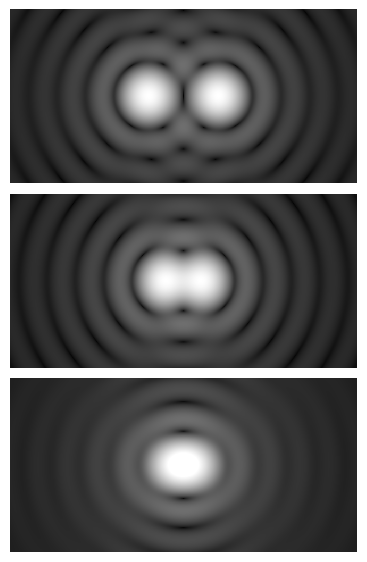
For typical, spatially incoherent imaging (such as Köhler-illuminated brightfield or fluorescence detection), a widely used estimate for the smallest resolvable lateral feature is the Rayleigh criterion:
Lateral resolution (Rayleigh):
d ≈ 0.61 · λ / NA
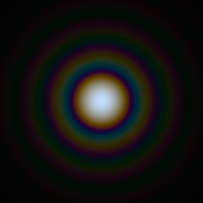
This image uses a nonlinear color scale (specifically, the fourth root) in order to better show the minima and maxima.
Artist: Spencer Bliven
Here, λ is the relevant wavelength in the specimen. In brightfield, you often consider the dominant illumination wavelength (e.g., green light around 550 nm). In fluorescence imaging, lateral resolution is governed by the emission wavelength of the fluorophore band you detect.
Axial (depth) resolution is poorer than lateral resolution in widefield microscopy because fewer high-angle rays contribute to sectioning along the optical axis. A common rule-of-thumb for widefield axial resolution is:
Axial resolution (widefield, order-of-magnitude):
Δz ≈ 2 · n · λ / NA²
These expressions set expectations for diffraction-limited performance. Real systems introduce aberrations, misalignment, and sampling limitations that can broaden the PSF. Nevertheless, NA and wavelength remain the first-order determinants of what details are physically resolvable, long before magnification becomes relevant. For a deeper look at the blur’s structure and how image contrast transfers from object to image, see The Airy Pattern, PSF, and MTF.
How Wavelength and Refractive Index Shape the Diffraction Limit
Diffraction depends on wavelength, so shorter wavelengths support finer resolution. Blue light (e.g., 450 nm) yields smaller d than red light (e.g., 650 nm) for a given NA. The refractive index n affects NA through NA = n sin(θ), enabling high-NA imaging when using immersion media with n near that of the objective’s front lens and the specimen mounting medium.
- Air objectives:
n ≈ 1.0. Common NA range up to ~0.95 for dry objectives. Practical resolution is limited by the small maximum sine-cone angle achievable in air. - Water-immersion objectives:
n ≈ 1.33. Often used for aqueous specimens to reduce mismatch at the specimen interface and to improve axial performance compared with air objectives. - Glycerol immersion:
n ≈ 1.47. Helpful for samples mounted in higher-index media, moderating spherical aberration due to index mismatch. - Oil immersion:
n ≈ 1.515(at green wavelengths for standard oils). Enables the highest NA values in conventional widefield systems, with objectives commonly reaching NA ~1.4.
Choosing the immersion medium is not just about pushing NA. Refractive index mismatch between the specimen mounting medium, the cover glass, and the objective front lens introduces spherical aberration, which broadens the PSF, reduces peak intensity, and lowers contrast—especially away from the focal plane. High-NA objectives often specify a cover glass thickness (commonly 0.17 mm for #1.5H coverslips) because even small deviations can meaningfully degrade resolution and contrast. Some objectives provide a correction collar that allows small adjustments for cover glass thickness variations (often in the ~0.13–0.21 mm range) or for imaging slightly into higher- or lower-index samples.
When comparing theoretical limits across different modalities, coherence also matters. Incoherent imaging (typical for brightfield with Köhler illumination and for fluorescence detection) supports a spatial-frequency cutoff approximately twice that of coherent imaging for the same pupil, which is why you commonly see the incoherent Rayleigh expression 0.61 λ/NA. For coherent systems (e.g., some laser-illuminated interferometric techniques), the frequency support and resolution criteria differ. For everyday transmitted brightfield and fluorescence, treat your system as largely incoherent on detection, and use the incoherent criteria throughout this article. For details on how illumination impacts coherence, see Illumination and Coherence.
The Airy Pattern, PSF, and MTF: Why Details Blur and How to Think About It
An ideal circular pupil turns a point source into a concentric ring pattern at the image plane, the Airy pattern. The bright central disk’s radius to the first minimum is proportional to 1.22 λ / (2 NA) in the object space, which leads directly to the Rayleigh criterion for two points: they are just resolved when the maximum of one Airy disk aligns with the first minimum of the other. Other criteria (Sparrow, Houston, Dawes) exist with slightly different thresholds, but the key idea is the same: a finite aperture creates structured blur that limits separability of nearby features.
Artist: SiriusB
The PSF is the image of a mathematical point, and the image of any object can be built by adding up (convolving) PSFs weighted by the object’s brightness distribution. Equivalently, in the frequency domain, the optical transfer function (OTF) describes how spatial frequencies pass (or attenuate). The modulus of the OTF is the modulation transfer function (MTF), often plotted from zero to the cutoff frequency. Three takeaways:
- Cutoff frequency (incoherent): An ideal diffraction-limited incoherent system passes detail up to about
f_c ≈ 2 NA / λ(in cycles per unit length). Features finer than this are severely attenuated and effectively lost. - Contrast rolls off before the cutoff: Even well below
f_c, contrast declines as frequency rises. Two structures of the same size can appear with different clarity if one sits near where the MTF is already low. - Aberrations shift and reduce the MTF: Spherical aberration, coma, and astigmatism lower contrast at intermediate frequencies more than they change the absolute cutoff. That is why an objective with the same nominal NA can produce different image quality if not matched to the cover glass and medium. See Depth of Field, Working Distance, and Cover Glass for practical constraints that affect aberration.
Because detection is finite in size (pixels), digital sampling also sets an upper bound on the spatial frequencies you can record without aliasing. The sampling bound is separate from, but must be chosen with respect to, the optical cutoff. This is covered in Magnification, Camera Pixel Size, and Nyquist Sampling.
Depth of Field, Working Distance, and Cover Glass: Hidden Constraints
High NA sharpens lateral and axial resolution, but it also tightens tolerances elsewhere in the system. Three practical constraints routinely shape real-world performance:
Depth of field decreases as NA increases
Depth of field (in object space) describes how much axial range appears acceptably sharp. For diffraction-limited imaging, DOF scales approximately inversely with NA² and linearly with wavelength and refractive index. A commonly used order-of-magnitude expression for widefield is:
DOF (object space, widefield, approx.):
DOF ∝ n · λ / NA²
Exact coefficients depend on definition (e.g., contrast thresholds and whether coherent or incoherent imaging is assumed). The important scaling is that pushing NA higher makes DOF shallower. This increases sensitivity to specimen tilt and thickness and can make focusing more demanding.
Working distance tends to shrink at higher NA
Working distance is the space between the objective’s front lens and the focal plane in the specimen. As NA increases, objectives generally require larger front elements and tighter lens groups closer to the sample, reducing working distance. Although there are long-working-distance objectives at moderate NA, at the highest NA values the trend is toward short working distances. This matters for thick or uneven samples, and for manipulations near the focal plane.
Cover glass thickness and index matching affect aberrations
High-NA objectives are often specified for a precise cover glass thickness, commonly 0.17 mm for #1.5H coverslips. Deviations from this value—whether from using a different coverslip class or tilting the coverslip—introduce spherical aberration, enlarging the PSF and reducing peak intensity. Immersion oil objectives are particularly sensitive: they assume a chain of materials with similar refractive indices (objective front lens, oil, cover glass, mounting medium) so wavefronts converge correctly. If you must image into media with refractive index far from oil, a water or glycerol immersion objective can reduce mismatch and preserve axial fidelity better than an oil lens at the same nominal NA.
Many high-NA objectives include a correction collar to compensate slightly for thickness differences and minor index mismatch. Adjusting the collar balances spherical aberration by redistributing blur between the center and periphery of the pupil. Using the collar should be done carefully and with suitable test features, but even without a step-by-step procedure, the principle is simple: tune for the sharpest, highest-contrast image while maintaining the specified cover glass class.
Illumination and Coherence: Brightfield, Fluorescence, and Structured Light
How you illuminate the specimen changes the coherence of light interacting with it, which in turn affects contrast formation and the applicable resolution criteria.
- Brightfield with Köhler illumination: Properly adjusted Köhler illumination creates a field that is approximately spatially incoherent at the specimen plane. Incoherence allows the image to be described by intensity convolution with the PSF, and the cutoff frequency is about
2 NA/λfor an ideal pupil. Most of the formulas in this guide assume this regime. - Fluorescence detection: Fluorescence emission is effectively spatially incoherent. Resolution depends on the emission wavelength and the detection NA. The dichroic mirror and emission filter isolate the emission band; the PSF and OTF should be considered at the emission wavelength.
- Coherent techniques: Methods like laser interferometry, holography, and some phase retrieval approaches operate under coherent or partially coherent conditions. The coherent cutoff frequency differs (approximately
NA/λfor an ideal pupil), and contrast responds differently to aberrations. - Structured or confocal illumination: Confocal detection modifies both excitation and detection PSFs, improving contrast and optical sectioning and narrowing the effective PSF compared with widefield. Structured illumination microscopy (SIM) uses patterned light and computational reconstruction to extend frequency support. These are specialized beyond the scope of this fundamentals overview, but they rest on the same PSF/OTF principles.
In practical widefield work, assuming incoherent detection is a robust starting point. For the purpose of sampling and magnification choice, you can then use the incoherent cutoff to set Nyquist criteria, as explained in Magnification, Camera Pixel Size, and Nyquist Sampling.
Magnification, Camera Pixel Size, and Nyquist Sampling in Digital Microscopy
Magnification does not improve optical resolution; it enlarges the image. However, digital imaging introduces a second, independent limit: how finely you sample the image with pixels. If your sampling is too coarse, you alias high-frequency detail into lower frequencies, creating misleading structure or erasing true fine detail—even if the optics could resolve it.
Linking pixel size to sample-plane sampling
A camera pixel of pitch p_cam images a region of the specimen whose size is approximately p_sample = p_cam / M_total, where M_total is the total magnification from specimen to sensor. In many infinity-corrected microscopes, M_total is the product of objective magnification and tube-lens or relay magnifications that project the intermediate image onto the camera sensor.
To avoid aliasing, the Nyquist-Shannon sampling theorem requires sampling at least twice the highest spatial frequency you wish to record. For an incoherent, diffraction-limited microscope with ideal pupil, the cutoff frequency is roughly f_c ≈ 2 NA / λ. Nyquist then demands:
Nyquist sampling at specimen:
p_sample ≤ 1 / (2 f_c) = λ / (4 NA)

Artist: Jacopo Bertolotti
Combining with the relationship p_sample = p_cam / M_total gives a practical target for magnification:
Minimum magnification for Nyquist:
M_total ≥ p_cam / (λ / (4 NA)) = 4 · NA · p_cam / λ
This expression is handy for checking whether a given camera and objective pair undersamples. Because real PSFs are not perfect and contrast near cutoff is low, many practitioners sample a bit finer than the strict cutoff criterion (e.g., aiming for ~2.3–3 samples across the smallest resolvable period). But λ / (4 NA) is a solid, widely used starting point for widefield sampling calculations.
Numerical examples
- Example A (widefield, green light): Suppose
λ = 550 nm(0.55 µm),NA = 0.95, and a camera withp_cam = 6.5 µmpixels. Thenp_sample ≤ 0.55 / (4 × 0.95) ≈ 0.145 µm. Required magnification:M_total ≥ 6.5 / 0.145 ≈ 44.8×. A 40× objective on a standard system would slightly undersample with 6.5 µm pixels; a 60× objective would meet or exceed Nyquist. - Example B (high-NA oil objective): With
λ = 550 nm,NA = 1.40, andp_cam = 6.5 µm, Nyquist demandsp_sample ≤ 0.55 / (4 × 1.4) ≈ 0.098 µm. ThenM_total ≥ 6.5 / 0.098 ≈ 66×. A 60×/1.40 oil objective paired with 6.5 µm pixels is close but slightly undersamples; a 100× objective oversamples, which is safe for preserving detail at the expense of more pixels per field. - Example C (small-pixel sCMOS): If
p_cam = 3.45 µmandNA = 1.40withλ = 550 nm, Nyquist requiresM_total ≥ 3.45 / 0.098 ≈ 35×. Here, a 40× objective sufficiently samples, and a 60× objective oversamples.
These examples illustrate why the right magnification depends on both NA and pixel size. Picking magnification solely by tradition (e.g., “always 40×”) can lead to undersampling with larger pixels or unnecessary oversampling with small pixels.
Field of view and sensor size
Increasing magnification to satisfy Nyquist reduces the field of view (FOV) at the sensor. Large-format sensors recover FOV but may require objectives and tube lenses with sufficient image circle to avoid vignetting and edge aberrations. Ensure your optics can cover the sensor format at the chosen magnification without unacceptable falloff or distortion.
Digital zoom versus optical magnification
Digital zoom enlarges pixels after sampling; it does not recover lost detail. If you undersample, no amount of digital enlargement will reconstruct high-frequency content. By contrast, proper optical magnification ensures that sufficient pixels are allocated to the finest details before the image is recorded.
Infinity-corrected systems and effective magnification
Many modern microscopes are infinity-corrected: the objective sends collimated light to a tube lens that creates the intermediate image. The objective’s nominal magnification assumes a specific tube lens focal length (e.g., 180 mm or 200 mm). If your system uses a different tube lens or adds relay optics, the effective magnification at the sensor can differ from the objective’s engraving. For sampling calculations, use the actual total magnification to the camera rather than the nominal objective value.
For a broader context on why sampling interacts with optical blur and contrast, revisit The Airy Pattern, PSF, and MTF. And for guidance on balancing NA against light budget and specimen compatibility, see Choosing Numerical Aperture.
Choosing Numerical Aperture: Contrast, Light Budget, and Sample Compatibility
Higher NA improves resolution and increases light collection, but it also brings trade-offs in depth of field, working distance, and sensitivity to alignment and aberrations. Selecting NA is a system-level choice involving your sample, illumination, required resolution, camera, and the practicalities of handling and mounting.

Artist: Happie1Soul
Light collection scales strongly with NA
For small to moderate collection angles, the solid angle (and thus collected signal) grows roughly with NA². This quadratic dependence means that even modest increases in NA can significantly boost signal. In fluorescence microscopy, where photons are precious, increasing NA can markedly improve signal-to-noise ratio (SNR) for the same exposure, assuming aberrations remain controlled.
Contrast and aberration sensitivity
High-NA systems are more sensitive to spherical aberration from refractive index mismatch and cover glass deviations. If you must image deep into a medium that differs substantially from the objective’s design medium, the effective resolution advantage of a higher NA lens can be compromised by aberration. In such cases, an immersion medium that better matches your sample (e.g., water immersion for aqueous samples) may outperform an oil objective with higher nominal NA, especially for axial fidelity.
Specimen and mounting considerations
- Cover glass dependence: If your application relies on standard #1.5H coverslips and thin, planar samples, oil-immersion high-NA objectives deliver outstanding lateral resolution and light-gathering.
- Thicker or index-mismatched samples: Water- or glycerol-immersion objectives mitigate mismatch and often provide better axial performance into the sample, with somewhat lower maximum NA.
- Clearance needs: If you need more space between lens and sample (e.g., for micromanipulation or uneven specimens), long-working-distance objectives with moderate NA can be the better choice, accepting reduced resolution but gaining practicality and safety margin.
Balancing NA with sampling and magnification
The choice of NA should be coordinated with your camera and magnification to meet Nyquist without overconstraining FOV and exposure times. A common strategy:
- Set a target wavelength band for your modality (illumination or emission).
- Choose the highest NA consistent with your sample’s medium and geometry.
- Compute the Nyquist-limited specimen pixel size
λ / (4 NA). - Given your camera pixel size, choose magnification to meet or slightly exceed Nyquist (see Magnification, Camera Pixel Size, and Nyquist Sampling).
This coordinated approach prevents common pitfalls like pairing a very high-NA objective with too little magnification on a large-pixel camera (aliasing) or pushing to extreme magnification on a small-format sensor (excessive oversampling with cramped FOV).
Common Misconceptions About Magnification and Resolution
- “More magnification means more detail.” Not beyond the optical resolution limit. Past a certain point, extra magnification only enlarges the blur—the image looks bigger but not sharper. The useful magnification range is set by the optics’ PSF and by sampling limits (see Magnification and Nyquist).
- “Numerical aperture and magnification are interchangeable.” They are not. NA determines resolution and light collection; magnification scales the image. Objectives with the same magnification can have very different NA and thus very different resolving power and brightness.
- “Shorter wavelength always wins.” Short wavelengths improve diffraction-limited resolution, but practical constraints such as specimen absorption, photodamage thresholds, and chromatic aberrations can offset the gains. Also, in fluorescence you are bound by the emission band of the fluorophore.
- “Any coverslip will do.” High-NA imaging assumes a specific cover glass thickness and refractive index environment. Using the wrong coverslip class or tilting it can noticeably degrade contrast and resolution, even if focus looks sharp at first glance (see Cover Glass Constraints).
- “Digital zoom fixes undersampling.” It does not. If you exceed the Nyquist limit at the specimen, aliased content is irretrievably lost or distorted in the recorded data.
Practical Calculations and Rules of Thumb
Below are concise, widely used relationships for diffraction-limited, incoherent imaging. They help you estimate limits and plan setups. Coefficients vary with precise definitions and criteria, but these serve well as first approximations.
Core relationships
- Lateral resolution (Rayleigh, incoherent):
d ≈ 0.61 λ / NA - Axial resolution (widefield, order-of-magnitude):
Δz ≈ 2 n λ / NA² - Cutoff spatial frequency (incoherent):
f_c ≈ 2 NA / λ - Nyquist specimen sampling:
p_sample ≤ λ / (4 NA) - Specimen pixel size from camera:
p_sample = p_cam / M_total - Minimum magnification for Nyquist:
M_total ≥ 4 NA p_cam / λ
Worked example: planning a 60× fluorescence setup
Suppose you are imaging green fluorescence with emission centered near λ = 520 nm, using a NA = 1.40 oil objective, and a camera with p_cam = 6.5 µm pixels. Compute specimen sampling and compare to Nyquist.
- Lateral Rayleigh:
d ≈ 0.61 × 0.52 µm / 1.40 ≈ 0.227 µm. - Nyquist specimen pitch target:
p_sample ≤ 0.52 / (4 × 1.40) ≈ 0.093 µm. - With 60×,
p_sample = 6.5 / 60 ≈ 0.108 µm, slightly coarser than Nyquist. With 100×,p_sample = 6.5 / 100 = 0.065 µm, safely finer than Nyquist.
If you must stay at 60× (e.g., for FOV or working distance), a smaller-pixel camera (e.g., p_cam ~ 3.45 µm) would meet Nyquist (3.45 / 60 ≈ 0.0575 µm), but note that smaller pixels collect fewer photons per pixel at the same irradiance. Exposure and noise characteristics must be considered alongside sampling.
Estimating depth of field
For widefield, a rough DOF estimate in object space is proportional to n λ / NA². For instance, with λ = 550 nm, n = 1.515, NA = 1.40, DOF is on the order of micrometers (e.g., sub-micrometer to a few micrometers depending on definition). The exact numeric factor depends on the criterion (e.g., contrast threshold, wavefront error), but the 1/NA² dependence consistently captures the trend that axial tolerance shrinks rapidly as NA increases.
Checking cover glass compatibility
Most high-NA objectives designed for coverslip use expect #1.5H cover glasses (~0.170 mm nominal thickness). If your sample uses a different thickness, a correction-collar objective can help compensate within a limited range; otherwise consider an objective designed for no coverslip (e.g., for dipping) or for thicker windows.
Rule-of-thumb summary
- Higher NA improves resolution roughly linearly and increases light collection roughly quadratically.
- Shorter wavelengths improve resolution but may reduce transmission and increase phototoxicity risk in live specimens (consider this contextually and ethically; this article remains educational and non-clinical).
- Match immersion medium to specimen refractive index when possible to limit spherical aberration and preserve contrast.
- Use Nyquist to select magnification for your pixel size; avoid relying on digital zoom to make up for undersampling.
- Respect cover glass specifications for high-NA objectives; small thickness errors matter.
For how these rules interact with camera and magnification choices, refer back to Magnification, Camera Pixel Size, and Nyquist Sampling.
Frequently Asked Questions
Is there a simple way to know if I am oversampling or undersampling?
Yes. Compute the Nyquist specimen pitch target λ/(4 NA) for your imaging wavelength and objective. Then compute your actual specimen pitch p_sample = p_cam / M_total. If p_sample is larger than the Nyquist target, you are undersampling and will lose fine detail and risk aliasing. If it is significantly smaller, you are oversampling, which preserves detail but increases the number of pixels per field and may reduce per-pixel signal. A moderate degree of oversampling is generally safe and often desirable for robust processing and display.
How does confocal microscopy change the resolution discussion?
Confocal microscopy modifies both the excitation and detection process using a focused spot and a pinhole, which rejects out-of-focus light and narrows the effective PSF compared with widefield. Lateral resolution can improve relative to widefield, and axial sectioning improves more strongly. The exact performance depends on pinhole size and optical configuration. Nevertheless, diffraction and NA still set the fundamental scale; confocal typically refines contrast and sectioning within those limits rather than overturning them. The same sampling logic applies: to record the improved detail, you must sample adequately at the specimen according to Nyquist.
Final Thoughts on Choosing the Right Resolution and NA
Resolution in optical microscopy rests on a small set of interconnected principles: diffraction sets the physical limit; numerical aperture and wavelength tune where that limit lies; aberrations and refractive index matching determine how close you get to it; and digital sampling decides whether your camera faithfully records what the optics deliver. Magnification, important as it is, should be selected to satisfy Nyquist for your NA and wavelength, not for its own sake.
When planning a setup or evaluating an image, ask four questions:
- What wavelength band am I imaging, and is my objective’s NA appropriate for the detail I need?
- Is the immersion medium and cover glass specification matched to the objective’s design to minimize aberrations?
- Does my total magnification and camera pixel size meet the Nyquist criterion at the specimen plane?
- Are field of view, working distance, and depth of field acceptable for my specimen geometry and task?
Answering these consistently will align your system with the physics of image formation. The payoff is visible: higher, truer contrast at fine scales and digital data that can be measured and processed with confidence. If you found this fundamentals guide helpful, explore our other articles linked in the Table of Contents and consider subscribing to our newsletter to receive future deep-dives on optical microscopy, sampling strategies, and practical optimization tips.

