What Is Urban Deep-Sky Astrophotography and Why It Works
Urban deep-sky astrophotography is the art and technique of capturing faint celestial objects—nebulae, galaxies, and star clusters—under light-polluted skies. Instead of escaping to pristine mountaintops, you use optics, filters, careful data acquisition, and computational processing to overcome city skyglow. The key idea is surprisingly simple: even though light pollution brightens the background, your target still emits light in characteristic ways you can isolate, enhance, and stack over time.
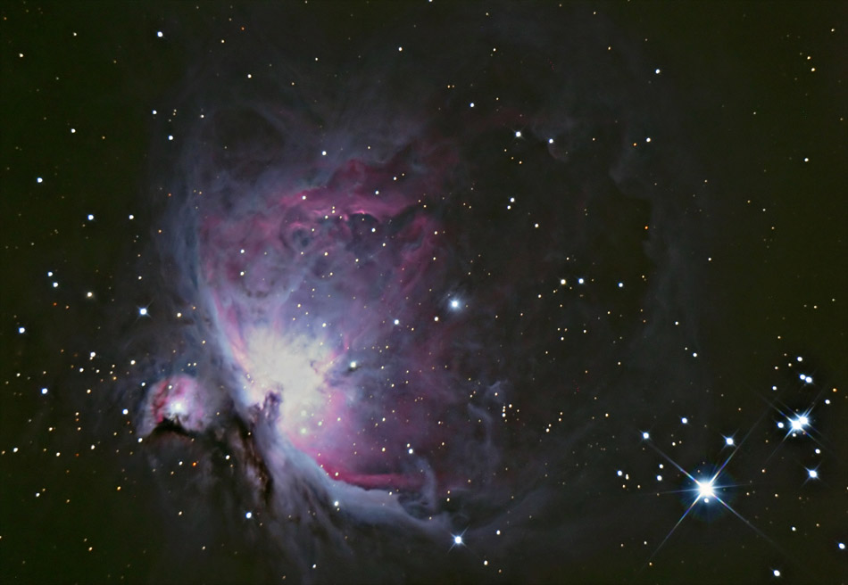
Artist: Rochus Hess
Modern sensors, precise tracking, and powerful software have reshaped what’s possible from balconies and backyards. With strategies like narrowband filtering, meticulous polar alignment and guiding, and long total integration times, you can build high signal-to-noise images that reveal structure, color, and subtle detail—right from Bortle 7–9 zones.
This guide distills practical, evidence-based methods for achieving strong results under city skies. We’ll cover gear choices, filters, photon management, exposure strategy, calibration and stacking, gradient control, color handling, and problem-solving. Whether you’re using a modest star tracker and lens or a guided equatorial mount and small refractor, you’ll find a repeatable workflow that scales with your ambitions.
Light Pollution Fundamentals: Bortle Scale, Skyglow, and SQM
Light pollution raises sky brightness, washing out low-contrast details and limiting the depth of your exposures. Understanding the metrics helps you plan effectively:
- Bortle Scale: A qualitative class from 1 (excellent dark sky) to 9 (bright inner city). Urban observers often work under Bortle 7–9.
- SQM (Sky Quality Meter) readings: Quantitative magnitude per square arcsecond. Dark skies are often 21–22 mag/arcsec². Typical bright suburban to city centers can be 18–20 or worse. Lower numbers mean brighter skies.
- Skyglow spectrum: Today’s urban skyglow is a mix of older sodium lamps and widespread white LEDs, which emit a broad continuum. This affects how well different filters work (see Filter Strategy).

Artist: Alejandro Sánchez de Miguel
Because light pollution chiefly adds a relatively uniform background, your camera captures target + skyglow + noise. You can treat the skyglow as contamination to be subtracted or suppressed with filters and gradient tools. The noise component averages down with stacking: SNR scales roughly with the square root of the total number of subexposures, all else equal. That’s why urban astrophotography often prizes total integration time above any other single variable.
Rule of thumb: Under light pollution, total hours dominate. Aim for multiple hours per target and plan for incremental improvement over several nights.
Essential Gear for City Imaging: Cameras, Optics, and Mounts
Equipment choices dramatically influence what you can accomplish from the city. The good news: success is possible with modest gear if you match your setup to the conditions and your goals. Here’s how to think about cameras, optics, and mounts.
Cameras: DSLR/Mirrorless, One-Shot Color CMOS, and Monochrome
- DSLR/Mirrorless: Popular entry choice. Unmodified cameras capture broadband targets and star fields well; modified (full-spectrum or H-alpha enhanced) models improve red nebula sensitivity. They pair nicely with lenses and small refractors.
- One-Shot Color (OSC) Astronomy CMOS: Thermally regulated cooling reduces dark current. Many modern OSC sensors have high quantum efficiency, low read noise, and good dynamic range. Combined with dual-band filters, OSC excels on emission nebulae under heavy skyglow.
- Monochrome CMOS/CCD: Maximum flexibility and efficiency in narrowband (H-alpha, OIII, SII) and LRGB imaging. Mono with a filter wheel excels at separating signal from skyglow, especially for dim structures. Complexity and cost are higher, but data quality can be exceptional from cities.
Optics: Fast Lenses, Refractors, and Reflectors
- Camera lenses (24–200 mm): Great for widefield targets like the North America Nebula region, Orion, or large HII complexes. Fast apertures (f/2–f/4) help build signal quickly; stop down slightly for better stars.
- Small refractors (60–100 mm aperture): A sweet spot for urban imaging. Apochromatic triplets or doublets with good color correction produce sharp stars. A field flattener or reducer-corrector simplifies processing and gives a wider, brighter field.
- Reflectors (e.g., 150–200 mm Newtonians): Bright images and fine resolution. Fast Newtonians (f/4–f/5) are efficient but require careful collimation and spacing for coma correctors. They can be great for brighter galaxies and planetary nebulae even from the city.
Mounts: Star Trackers vs. Equatorial Mounts
- Star trackers: Portable and budget-friendly. Ideal for lenses up to ~135–200 mm. Accurate polar alignment becomes critical; guiding is optional but beneficial for longer subs. Trackers are an excellent way to begin urban astrophotography.
- Equatorial mounts: For telescopes and longer focal lengths, a well-tuned EQ mount with autoguiding is the foundation for sharp data. Capacity headroom, belt drives, and good periodic error control improve tracking reliability.

Artist: Gustaaf Prins from Haarlem, The Netherlands
Whatever you choose, be disciplined about setup repeatability: balance the mount, secure cables, ensure correct backfocus, and dither between subexposures. These fundamentals often beat out expensive upgrades.
Filter Strategy: Broadband, Dual-Band, and True Narrowband
Filters are among the most powerful tools for urban imagers. Choose based on your camera and target type:
Broadband and Light Pollution (LP) Filters
- UV/IR cut: Essential for some sensors/telescopes to maintain sharp star profiles by blocking out-of-focus infrared and ultraviolet light.
- General LP filters: Historically designed to suppress emission from sodium and mercury lamps. Their effectiveness is reduced under white LED-dominated skies, which emit a broad spectrum. They still help somewhat, but expect modest gains and possible color shifts.
- Luminance (L) filters for mono: Under heavy LP, using a pure L filter often leads to bright gradients. Consider relying more on narrowband or gathering L under darker skies. For galaxies, you can still collect L in the city but prepare for aggressive gradient management.
Dual-Band and Multi-Band Filters for OSC
Dual- and tri-band filters isolate common nebular emission lines—typically H-alpha (656.3 nm) and OIII (500.7 nm), sometimes SII (672.4 nm). These filters are highly effective in urban environments because they reject most broadband skyglow while passing the target’s line emissions.
- Bandwidth: Narrower (e.g., ~5 nm) generally rejects more skyglow and improves contrast but may dim stars and require longer exposures. Slightly wider (~7–10 nm) can improve star colors and signal throughput.
- Target types: Emission nebulae benefit hugely. Reflection nebulae and broadband galaxies do not respond well to these filters because they emit continuum light, which the filter blocks.
True Narrowband for Monochrome Cameras
Mono cameras with individual H-alpha, OIII, and SII filters allow precise control. Under Bortle 7–9, narrowband can feel like magic: your images cut through the glow to reveal delicate filaments and shock fronts. You’ll combine channels into palettes like HOO (H-alpha, OIII, OIII) or SHO (SII, H-alpha, OIII). See Color Calibration, Stars, and Narrowband Combinations for mapping strategies.

Tip: If you use an OSC with a dual-band filter, consider capturing a separate short set of RGB stars without the filter on a moonless night. You can later replace dual-band stars with natural-color RGB stars during processing.
Planning Targets and Sessions from the City
Good planning maximizes your usable signal when fighting the city glow.
Target Selection Under Light Pollution
- Best bets: Emission nebulae (HII regions, supernova remnants, planetary nebulae) respond well to narrowband filtration. Open clusters can also work because they stand out against the background, especially with a short focal length.
- Challenging targets: Reflection nebulae, dark nebulae, and faint galaxy halos demand dark skies. You can attempt brighter galaxies in the city, but expect to devote many hours and meticulous gradient removal.

Altitude, Transit, and Seasonality
- Altitude: Aim to image when the target is high in the sky, ideally near meridian transit. This reduces atmospheric extinction and improves resolution.
- Seasonality: Map targets by season to get the best windows (e.g., Orion in winter, Cygnus in summer for Northern Hemisphere). A planning tool or planetarium app can help you pick efficient sequences.
- Moon phase: Narrowband lets you work even during bright Moon, but avoid imaging close to the Moon to reduce gradients. For broadband, stick to darker nights or when the Moon is below the horizon.
Framing, Field of View, and Composition
Use FOV calculators to simulate framing with your sensor and focal length. Consider including foreground stars and nearby structures for context. Don’t be afraid to rotate the camera to align the target’s long axis along the frame diagonal. Planning composition pays off later when you process and crop.
Accurate Polar Alignment, Guiding, and Dithering
Accurate tracking makes or breaks sharp imaging, especially as focal length increases. Three pillars—polar alignment, guiding, and dithering—form the backbone of reliable subexposures.
Polar Alignment Methods
- Polar scope alignment: Calibrate for your location and place Polaris (or Sigma Octantis in the south) at the correct clock angle in the reticle. Ensure the mount is level and the polar scope is collimated.
- Software-assisted alignment: Many capture suites provide plate-solve-based polar alignment. These routines rotate the mount a small amount, plate-solve the star field, and compute the polar offset, guiding you to adjust altitude and azimuth. It’s accurate and quick, even where Polaris is obstructed.
- Drift alignment: The classic method using star drift near the meridian and celestial equator. Time-consuming but precise if you lack a view of the pole.
Autoguiding Basics
- Multi-star guiding: Modern autoguiding analyzes several guide stars to average out seeing effects. It improves stability over single-star approaches.
- Guide scope vs. OAG: A short guide scope works well at short to moderate focal lengths. Off-axis guiders (OAG) sample the main optical path, minimizing differential flexure—helpful for longer focal lengths.
- Guiding cadence: Sample frequently enough to track mount error but not so fast that you chase seeing. Typical cadences range from 1–3 seconds, adjusted to conditions.
Dithering to Beat Pattern Noise
Dithering randomly shifts the telescope a small amount between subexposures. It’s one of the most effective tools against banding and walking noise (pattern noise that drifts with tracking). A displacement of ~10–20 pixels with a short settle time is a good starting point. Most capture software can coordinate dithers automatically with your guiding program. Make sure to enable it, especially if you see streaky background artifacts after stacking.
Exposure Time, Gain/ISO, and Total Integration
Under urban skies, exposure strategy balances three competing factors: dynamic range, sky background brightness, and read noise. Your goal is to expose long enough that sky background rises above read noise (“sky-limited”), but not so long that you saturate bright stars or clip nebular cores.
Subexposure Length and Histogram Placement
- Histogram peak: A common heuristic is to place the background peak some distance above the left edge of the histogram—roughly 20–30% from the left for broadband, possibly lower for narrowband where the sky is darker through the filter.
- Adapt to conditions: In Bortle 8–9, broadband subexposures may need to be relatively short to avoid saturation (e.g., tens of seconds to a couple of minutes). Narrowband subs can often be longer due to heavy light rejection (several minutes each, depending on tracking quality).
Gain and ISO
- Unity gain (CMOS): Setting gain near the camera’s unity gain often balances read noise and dynamic range. If bright stars clip too easily, lower the gain; if read noise dominates, raise it slightly. Consult your camera’s characteristics.
- ISO (DSLR/Mirrorless): ISO does not change the camera’s native sensitivity, but affects read noise and dynamic range as recorded in RAWs. Many cameras perform well around manufacturer-recommended ranges; avoid extremely high ISO that compresses highlights.
Total Integration Time and SNR
Stacking N subexposures increases SNR ~ √N. At fixed sub length, doubling total integration from 2 to 4 hours improves SNR by ~41%. More total time is nearly always beneficial under light pollution, which raises background noise that stacking averages down.
Image scale matters for resolution and guiding. A useful relation for pixel scale is:
arcsec_per_pixel = 206.265 * pixel_size_microns / focal_length_mmMatching your sampling to typical seeing (often ~2–3 arcseconds in many locations) helps you choose focal length and pixel size. Oversampling excessively can waste SNR; undersampling can limit detail. A range of roughly 1–2.5 arcsec/pixel is a practical target for many urban setups.
Calibration Frames, Stacking, and Gradient Control
Calibration frames and robust stacking are essential to combat noise and artifacts that light pollution amplifies. Combine this with dedicated gradient control to recover a flat background.
Calibration Frames: Bias, Darks, Flats (and Dark Flats)
- Bias: Very short exposures with the lens cap on, capturing readout pattern. For some modern CMOS cameras, bias frames can be replaced by matching dark flats due to sensor behavior; consult your camera’s guidance.
- Darks: Same exposure time, temperature, and gain as your lights, but with no light. They model thermal noise and hot pixels. Cooled cameras make dark libraries practical; for uncooled cameras, try to match ambient temperature as closely as possible.
- Flats: Compensate for vignetting and dust shadows. Create with a uniform light source (flat panel, dawn/dusk sky, t-shirt method) at the same focus and optical train configuration as your lights. Correct flats are especially crucial with filters and fast optics.
- Dark flats: For cameras where traditional bias frames cause issues, dark flats match the flat exposure time to model read noise more accurately.
Stacking Tools and Rejection Algorithms
- Software: Popular options include DeepSkyStacker, Siril, Astro Pixel Processor, and PixInsight. They handle calibration, registration, normalization, and integration.
- Weighting and normalization: Quality-weight frames by FWHM, eccentricity, and noise. Normalize background levels to prevent gradients from skewing the integration.
- Outlier rejection: Sigma-clipping, Winsorized sigma, and linear fit clipping remove satellites, airplanes, and cosmic rays. Dithering improves rejection effectiveness by decorrelating pattern noise.
Gradient Control and Background Extraction
Light-polluted images feature gradients from streetlights, the Moon, or local reflections. Dedicated background extraction tools place sample points in empty sky and model the gradient surface to subtract it. Automatic and dynamic methods both work; dynamic approaches give more control over complex gradients. Aim for a neutral, smooth background without erasing faint nebulosity—use masks and evaluate results at multiple stretches.
Tip: Perform gradient removal in the linear stage (before strong stretching) to avoid baking gradients into the signal.
Color Calibration, Stars, and Narrowband Combinations
City imaging complicates color. Streetlights and LED spectra distort white balance and star colors. Careful calibration and combination strategies reintroduce realism or aesthetic intent.
Color Calibration and Star Management
- Photometric or reference-based calibration: Tools can match star colors to catalogs or use reference regions to neutralize the background and set white balance. This is especially helpful after gradient correction.
- Star reduction: Morphological operations or star-specific tools can modestly shrink stars, balancing them against bright nebulae. Apply conservatively to avoid halos or unnatural profiles.
- RGB stars with dual-band data: Replace dual-band stars with short RGB star exposures to restore natural hues and mitigate green/cyan dominance from OIII. Register and mask stars for clean replacements.
Narrowband Combinations: HOO and SHO
- HOO mapping: Assign H-alpha to red, OIII to green and blue. This yields classic red/teal palettes for emission nebulae with OSC dual-band or mono filters.
- SHO mapping: Assign SII to red, H-alpha to green, OIII to blue. This “Hubble palette” highlights ionization structure but may require careful color balancing to tame green dominance.
- OSC dual-band synthesis: With OSC data, you can extract an H-like channel (red-weighted) and an O-like channel (green+blue weighted), then mix for HOO. Add a synthetic SII only if supported by additional data; avoid fabricating channels without measurement.
Whether you pursue naturalistic color or creative palettes, document your choices. The palette you pick conveys physical information (e.g., where shocks or ionization fronts dominate) and aesthetic tone.
Noise Reduction, Deconvolution, and Artifact Avoidance
Light pollution boosts background noise, making denoising a critical step. Used carefully, modern multi-scale methods preserve structure while smoothing the background. Overused, they smear detail and produce plasticky textures.
Noise Reduction Strategy
- Work in linear where possible: Some denoisers work best in the linear stage, guided by noise estimates and masks.
- Masking: Protect stars and bright structures with luminance and range masks. Apply stronger noise reduction to faint background regions.
- Multi-scale approach: Wavelet or multi-scale transforms address noise differently across small, medium, and large structures. Iterate lightly and evaluate at 100% to avoid over-smoothing.
Deconvolution and Sharpening
- PSF estimation: Derive a point-spread function from representative stars if your software supports it. A good PSF improves deconvolution accuracy.
- Star masks and ringing control: Constrain deconvolution with masks to reduce halos and ringing around bright stars. Conservative parameters are safer than aggressive ones that create artifacts.
- Final micro-contrast: After stretching, modest local contrast enhancements can make filaments pop. Keep a light touch and compare before/after frequently.
Example Urban Imaging Workflows (Widefield and Telescope)
Here are two practical, scalable workflows that demonstrate how to put the pieces together under city skies.
Workflow A: Widefield Dual-Band with a Star Tracker
- Setup: Mirrorless or OSC camera + 85–135 mm lens + dual-band filter + star tracker.
- Targets: Emission nebulae complexes (e.g., Cygnus region, Rosette/Monoceros, Orion).
1) Level tripod, rough polar alignment with app.
2) Attach lens and dual-band filter; focus with Bahtinov mask or live view on a bright star.
3) Polar align precisely (software-assisted if available).
4) Acquire 120–300s subs (as tracking allows) for 2–6 hours total.
5) Dither every 1–3 frames.
6) Capture calibration: darks matching sub length & temperature; flats; dark flats if needed.
7) Stack with sigma-clipping, weight by FWHM/eccentricity.
8) Gradient removal in linear stage.
9) Extract H- and O-like channels from the OSC data; mix HOO.
10) Light multi-scale denoise; modest star reduction.
11) Optional: Shoot 5–10 minutes of RGB stars without the filter on a dark night and replace stars.
12) Final stretch, color balance, and micro-contrast.
Workflow B: Small Refractor + Monochrome Narrowband on an EQ Mount
- Setup: 60–100 mm apochromatic refractor + mono CMOS + filter wheel (H-alpha, OIII, SII) + autoguiding.
- Targets: Planetary nebulae, supernova remnants, HII regions in Bortle 7–9.
1) Balance mount; route cables to avoid snags; precise polar alignment.
2) Autoguide with multi-star; dither between subs.
3) Capture 5–10 minute subs per filter (conditions/seeing may dictate shorter):
   - H-alpha: prioritize for structure (e.g., 3–6 hours)
   - OIII and SII: 2–4 hours each as needed
4) Build master darks and flats per filter; calibrate lights.
5) Register and integrate each channel; inspect for tilt/focus issues.
6) Gradient removal for each channel; linear denoise if needed.
7) Combine into HOO or SHO; balance colors and protect stars with masks.
8) Gentle deconvolution on the luminance (e.g., H-alpha or a synthetic blend).
9) Final stretch, star reduction, and targeted contrast enhancements.
These outlines translate readily to other combinations, such as OSC through a small refractor or mono with RGB filters. The core is consistent: stable tracking, sensible exposures, thorough calibration, and careful color handling.
Troubleshooting Common Urban Imaging Problems
City imaging amplifies technical foibles. Here are frequent issues and straightforward remedies.
- Walking noise/banding: Enable dithering; increase dither amplitude; ensure darks match temperature and exposure; consider a different stacking rejection method.
- Amp glow (in some sensors): Use matched darks; investigate camera settings that mitigate glow; modern calibration should remove it when parameters match well.
- Star bloating and halos: Check focus and optical spacing; stop down fast lenses slightly; some filters introduce halos around bright stars—consider different filters or process halos with targeted masks.
- Coma/field curvature: Use a corrector or flattener matched to your telescope; verify backfocus distance carefully.
- Tilt/backfocus error: Look for asymmetric star shapes across corners. Adjust tilt plates or spacers to square the sensor to the optical axis.
- Guiding oscillations: Balance the mount slightly east-heavy; reduce aggressiveness if you’re chasing seeing; verify polar alignment and mechanical play.
- Gradient overcorrection: When background extraction removes nebula, increase sample protections, place samples only in blank sky, and use gentler parameters. Undo and iterate—don’t force a model onto your data.
- Color casts under LED lighting: Apply photometric calibration or neutralize the background with well-placed reference points. Replace stars with RGB data if dual-band skewed them.
Frequently Asked Questions
Can I photograph galaxies from the city?
Yes, but it’s more challenging than emission nebulae. Galaxies emit broadband light, so narrowband filters don’t help much. Under Bortle 7–9, you’ll likely need long total integration (many hours), careful gradient removal, and conservative stretching to reveal faint outer structures. Shorter focal lengths capture galaxies small in the frame; longer focal lengths can resolve details but demand tighter tracking and guiding. Prioritize brighter galaxies and consider acquiring additional time over multiple nights. If you also travel occasionally, one practical approach is to capture high-SNR luminance from a darker site and gather color from the city, then combine the datasets in processing.
Do I need a monochrome camera to succeed?
No. Many urban imagers produce excellent results with one-shot color cameras and dual-band filters, especially on emission nebulae. Monochrome systems do provide advantages—greater flexibility, efficiency in narrowband, and cleaner separation of signal from skyglow—but they add complexity and cost. A solid OSC workflow, rigorous tracking, smart exposure strategy, and disciplined calibration/stacking can deliver compelling images from city balconies and rooftops.
Final Thoughts on Choosing the Right Urban Astrophotography Approach
Urban deep-sky imaging is a balance of physics, engineering, and patience. You contend with skyglow, gradients, and variable seeing, yet modern sensors, narrowband filters, and robust processing unlock rich results. The most reliable path combines the following:
- Match your gear to the environment: fast optics and precise mounts; OSC + dual-band for simplicity or mono narrowband for control.
- Prioritize emission nebulae and high-altitude windows; plan around Moon and target transit (Planning Targets and Sessions).
- Invest in technique: polar alignment, guiding, and dithering (Alignment and Guiding).
- Expose smartly: aim for sky-limited subs and build hours of integration (Exposure Strategy).
- Process methodically: calibrate rigorously, remove gradients early, keep color grounded, and apply denoise/sharpening with restraint (Calibration and Noise Reduction).
From an apartment window or a city rooftop, you can produce images that illuminate stellar nurseries, supernova remnants, and galactic structure. Start with a simple setup, iterate deliberately, and let stacking work in your favor. If you enjoyed this guide, explore our related articles on capture workflows and processing fundamentals, and subscribe to our newsletter for future in-depth tutorials and target recommendations.
