Table of Contents
- What Is Optical Sampling in Digital Microscopy?
- Diffraction-Limited Resolution: Abbe, Rayleigh, and OTF
- Nyquist Sampling Criteria for Microscope Cameras
- Relating Sensor Pixel Size, Magnification, and Sample Scale
- Worked Examples for Common Objectives and Sensors
- Field of View, Sampling, and Information Throughput
- Pixel Binning, Color Filter Arrays, and Signal-to-Noise
- Point Spread, Airy Patterns, and Modulation Transfer
- Calibrating Image Scale and Verifying Sampling in Practice
- Common Pitfalls: Empty Magnification, Over- and Under-Sampling
- Frequently Asked Questions
- Final Thoughts on Matching Camera Sampling to Microscope Optics
What Is Optical Sampling in Digital Microscopy?
When a microscope image is captured by a digital camera, a continuous optical image is converted into a discrete grid of pixels. This conversion is called sampling. Each pixel measures the average light intensity over a small area of the sensor, and the arrangement of these pixels determines how faithfully spatial detail from the specimen is recorded. The central question for any digital microscopy setup is simple but consequential: Are the camera pixels small enough, relative to the microscope’s resolving power, to capture all the spatial detail without aliasing?
Good sampling requires the camera’s pixel pitch (projected to the specimen plane) to be sufficiently fine compared to the smallest features the optics can resolve. If you sample too coarsely, high-frequency detail “folds” into lower frequencies, producing spurious patterns (aliasing) and a loss of true resolution. If you sample far more finely than necessary, you usually do not gain additional optical detail; instead, you spread the same information across many pixels, which can reduce per-pixel signal-to-noise and increase data volume. Striking the right balance is the essence of Nyquist sampling in microscopy.

Attribution: Pixelmaniac pictures
Three parameters govern this balance:
- Numerical Aperture (NA) of the objective, which sets the optical system’s resolving power and spatial frequency bandwidth.
- Wavelength (λ) of light used for imaging, which influences diffraction and resolution directly.
- Effective magnification (M) between specimen and camera sensor, which scales how object-space details map onto sensor pixels.
Understanding how NA, λ, and M interact with sensor pixel size is fundamental. This article builds from first principles—diffraction and the optical transfer function—to derive practical rules for choosing magnification and camera pixel size, illustrate typical configurations with numerical examples, and highlight common pitfalls like empty magnification and undersampling.
Diffraction-Limited Resolution: Abbe, Rayleigh, and OTF
In brightfield and widefield fluorescence microscopy with incoherent or partially coherent illumination, the ability to distinguish fine detail is set by diffraction and the objective’s numerical aperture (NA). NA is defined by NA = n · sin(θ), where n is the refractive index of the imaging medium (e.g., air ~1.0, water ~1.33, immersion oil ~1.515) and θ is the half-angle of the cone of light accepted by the objective. Higher NA generally means better resolution because more of the diffracted light from the specimen is captured.
Common resolution criteria include:
- Abbe limit (cutoff frequency): For incoherent imaging, the optical transfer function (OTF) has a spatial frequency cutoff given by
ν_c ≈ 2·NA/λ(cycles per unit length in object space). Spatial frequencies above this cutoff are not transmitted by the objective. - Rayleigh criterion (lateral): Two point sources are considered resolvable when the principal maximum of one Airy pattern coincides with the first minimum of the other. A commonly used estimate for lateral resolution is
δ_R ≈ 0.61·λ/NA(distance in object space).
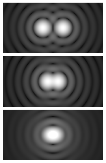
Attribution: Spencer Bliven
The OTF-based view is especially powerful for digital imaging because it connects directly to sampling theory: if the optics transmit spatial frequencies up to ν_c, then the camera must sample at least twice that frequency (Nyquist) to capture all transmitted detail without aliasing. We will return to this point in Nyquist Sampling Criteria and use it to derive object-side pixel size limits.
A practical note on wavelength: most microscopy scenes are broadband in brightfield, and many fluorescence experiments use well-defined emission bands. Because resolution scales with λ, working at shorter wavelengths improves resolution. Many calculations use a representative green wavelength (e.g., 520–550 nm) for white-light systems, or the band-appropriate effective wavelength for fluorescence. When calculating sampling requirements, pick a wavelength representative of the information you wish to preserve, and be consistent across your analysis.
Key takeaway: NA and wavelength together define both the size of the smallest resolvable features and the highest spatial frequencies the optics can deliver. Sampling must meet or exceed this optical bandwidth to faithfully digitize the image.
Nyquist Sampling Criteria for Microscope Cameras
The Nyquist–Shannon sampling theorem states that to capture a band-limited signal without aliasing, the sampling frequency must be at least twice the highest frequency present. Translating this into microscopy, where the optical system transmits up to an OTF cutoff ν_c ≈ 2·NA/λ (in cycles per unit length in object space), the sampling interval in object space p_obj (the pixel pitch projected to the specimen plane) must satisfy:
p_obj ≤ 1 / (2·ν_c) = λ / (4·NA)
This criterion ensures that all spatial frequencies up to the optical cutoff are sampled at or above Nyquist, preventing aliasing of the highest frequencies passed by the objective. It is a compact and robust rule for system design. Because it is derived from the OTF cutoff, it is somewhat stricter than a rule based directly on the Rayleigh criterion. For comparison, if you scheduled sampling to place roughly two samples across a Rayleigh-limited feature, you would set:
p_obj ≤ δ_R / 2 ≈ 0.61·λ / (2·NA) ≈ 0.305·λ/NA
This Rayleigh-based limit (~0.305·λ/NA) is more permissive than the OTF-based Nyquist limit (λ/(4·NA) = 0.25·λ/NA). The difference reflects that Rayleigh addresses a specific visibility threshold between two point sources, whereas the OTF criterion guards against aliasing across the full transmitted bandwidth. When in doubt, use the stricter OTF-based expression, especially for quantitative imaging or when preserving edge contrast and fine textures near the system’s resolution limit matters.
You will also see practical heuristics such as “sample with ~2–3 pixels across the smallest resolvable feature” or “use object-side pixel size of ~0.3–0.5·λ/NA.” These can work, but their precise meaning depends on which resolution criterion one adopts. The OTF-derived limit is explicit and easy to compute, making it the preferred design rule for avoiding aliasing.
- Nyquist-safe design rule (object side):
p_obj ≤ λ / (4·NA) - Rayleigh-based rule of thumb:
p_obj ≤ 0.305·λ / NA
Because p_obj is the sensor pixel pitch divided by the effective magnification (see Relating Sensor Pixel Size, Magnification, and Sample Scale), you can meet these limits either by choosing smaller pixels on the camera, by increasing magnification, or by a combination of the two. Each approach has trade-offs explored later in Field of View, Sampling, and Information Throughput and Pixel Binning, Color Filter Arrays, and Signal-to-Noise.
Relating Sensor Pixel Size, Magnification, and Sample Scale
The key practical relationship linking the camera and the specimen is:
p_obj = p_sensor / M_eff
where p_sensor is the camera’s physical pixel size (e.g., 3.45 µm or 6.5 µm) and M_eff is the total lateral magnification from the specimen to the sensor. In infinity-corrected microscope systems, the effective magnification is the product of the objective’s nominal magnification and the ratio of the actual tube lens focal length to the objective’s design tube lens focal length. For example:
- Effective magnification:
M_eff = M_obj · (f_tube / f_design)
If a 20× objective is specified for a 200 mm tube lens, and you use a 200 mm tube lens, then M_eff ≈ 20×. If you use a 180 mm tube lens with that same objective, then M_eff ≈ 20 × (180/200) = 18×. The design tube length is given by the objective’s specification (e.g., 200 mm is a common modern standard), and staying with the design value preserves the nominal magnification.
Rearranging the Nyquist-safe object-side rule from Nyquist Sampling Criteria, we can compute the magnification required to achieve Nyquist with a given sensor pixel size:
M_req ≥ p_sensor / p_obj_max = p_sensor / (λ / (4·NA)) = (4·NA·p_sensor) / λ
This equation is very useful for planning. With known NA, wavelength, and pixel size, you can estimate the magnification needed to sample at or above Nyquist. It also makes clear that, all else equal, higher NA optics require higher magnification (or smaller sensor pixels) to satisfy Nyquist, because the optics deliver higher spatial frequencies.
Another related perspective is the size of the Airy disk at the sensor. The lateral size of the diffraction-limited image of a point (Airy pattern) scales with magnification and NA. A common expression for the Airy disk diameter at the sensor is:
d_image ≈ 1.22 · λ · M_eff / NA
A sensible sampling guideline is to place at least ~2–3 pixels across the Airy disk diameter in the image plane. This is consistent with the object-side Nyquist limits after accounting for magnification.
Practical shortcut: For a given objective NA and an assumed wavelength (e.g., λ ≈ 0.55 µm for green), you can compute
M_reqwith the formula above and compare it to your available objective magnifications. IfM_effis belowM_req, consider either increasing magnification or selecting a camera with smaller pixels to meet Nyquist.
Worked Examples for Common Objectives and Sensors
The following examples illustrate how to apply the formulas. They assume an infinity-corrected system using a tube lens that preserves the objective’s nominal magnification, and a representative green wavelength λ = 0.55 µm (550 nm) for computation. When your imaging wavelength differs substantially (e.g., deep red fluorescence at ~650 nm, or near-UV at ~400 nm), redo the arithmetic with your chosen λ.
Example A: 10×/0.25 objective with a 6.5 µm pixel camera
- Given: NA = 0.25, λ = 0.55 µm, p_sensor = 6.5 µm
- Nyquist object-side limit:
p_obj_max = λ / (4·NA) = 0.55 / (4·0.25) ≈ 0.55µm - Required magnification:
M_req = (4·NA·p_sensor)/λ = (4·0.25·6.5)/0.55 ≈ 11.8×
With a 10× objective (assuming the nominal magnification is achieved), p_obj = 6.5 / 10 = 0.65 µm, which is slightly larger (coarser) than the 0.55 µm Nyquist limit. That means the system is a bit undersampled at the highest spatial frequencies. Using a 12×–13× effective magnification would meet the Nyquist criterion, or using a camera with smaller pixels (e.g., 4.5 µm) at 10× would also satisfy it. In practice, for modest-NA objectives like 10×/0.25, a 6.5 µm pixel at 10× is usable but is not strictly Nyquist for green light.
Example B: 20×/0.45 objective with a 6.5 µm pixel camera
- Given: NA = 0.45, λ = 0.55 µm, p_sensor = 6.5 µm
- Nyquist object-side limit:
p_obj_max = 0.55 / (4·0.45) ≈ 0.306µm - Required magnification:
M_req ≈ (4·0.45·6.5)/0.55 ≈ 21.3× - Actual at 20×:
p_obj = 6.5 / 20 = 0.325µm
At 20×, the object-side pixel size is 0.325 µm, very close to the Nyquist limit of 0.306 µm. This configuration is nearly Nyquist for λ = 0.55 µm and will generally capture fine detail with minimal aliasing. A slight increase in magnification (or using a 3.45 µm pixel camera) ensures a margin of safety.
Example C: 40×/0.75 objective with a 6.5 µm pixel camera
- Given: NA = 0.75, λ = 0.55 µm, p_sensor = 6.5 µm
- Nyquist object-side limit:
p_obj_max = 0.55 / (4·0.75) ≈ 0.183µm - Required magnification:
M_req ≈ (4·0.75·6.5)/0.55 ≈ 35.5× - Actual at 40×:
p_obj = 6.5 / 40 = 0.1625µm
At 40×, p_obj is 0.1625 µm, which is finer than the Nyquist limit. This configuration oversamples (good for preserving detail, at the cost of data volume). With NA 0.75 and 6.5 µm pixels, 40× satisfies Nyquist comfortably.
Example D: 60×/1.40 oil objective with a 6.5 µm pixel camera
- Given: NA = 1.40, λ = 0.55 µm, p_sensor = 6.5 µm
- Nyquist object-side limit:
p_obj_max = 0.55 / (4·1.40) ≈ 0.098µm - Required magnification:
M_req ≈ (4·1.40·6.5)/0.55 ≈ 66.2× - Actual at 60×:
p_obj = 6.5 / 60 ≈ 0.108µm
At 60×, the system is slightly undersampling relative to the OTF-based Nyquist criterion at λ = 0.55 µm. Moving to 63×–70× effective magnification would bring it on target, or a camera with smaller pixels (e.g., ~4 µm) at 60× would also meet Nyquist. Note that if your emission is in the red (longer λ), the Nyquist requirement is less strict, and 60× may suffice; conversely, at shorter wavelengths it becomes more demanding.
Example E: 100×/1.30 oil objective with a 3.45 µm pixel camera
- Given: NA = 1.30, λ = 0.55 µm, p_sensor = 3.45 µm
- Nyquist object-side limit:
p_obj_max = 0.55 / (4·1.30) ≈ 0.106µm - Required magnification:
M_req ≈ (4·1.30·3.45)/0.55 ≈ 32.7× - Actual at 100×:
p_obj = 3.45 / 100 = 0.0345µm
Here the system is heavily oversampling relative to the Nyquist limit—there is no additional optical detail to justify such fine sampling. While oversampling is safe from an aliasing perspective, it increases data size and may reduce per-pixel SNR for a given exposure. Depending on your goals (e.g., localization precision, deconvolution, or quantitative analysis), this can still be beneficial, but it is not required for resolving power.
These examples underscore an important point: it is the combination of NA, wavelength, pixel size, and magnification that determines if your setup is Nyquist-adequate. Where possible, design around the rule in Nyquist Sampling Criteria and then consider trade-offs using the guidance in Field of View, Sampling, and Information Throughput and Pixel Binning, Color Filter Arrays, and Signal-to-Noise.
Field of View, Sampling, and Information Throughput
Meeting Nyquist is not the only design objective. You also need adequate field of view (FOV) to cover your region of interest, and you may want high frame rates or manageable file sizes. These considerations interact in predictable ways:
- Increasing magnification reduces object-side pixel size (helping sampling) but proportionally shrinks the FOV on a given sensor. For a fixed sensor size, doubling magnification halves the FOV width and height.
- Smaller sensor pixels improve sampling at the same magnification without sacrificing FOV, but may increase read noise density or reduce full-well capacity per pixel, depending on sensor design.
- Sensor size affects total FOV. A larger sensor with the same pixel size provides a wider FOV at a given magnification—but may demand higher-quality optics to maintain flatness and correction across the field.
- Frame rates and data volume scale with pixel count and bit depth. Oversampling by a large factor may constrain acquisition speed or storage.
From an “information throughput” standpoint, a balanced design matches the optical bandwidth and sensor sampling while keeping the FOV large enough for the task. For tiled imaging or scanning workflows, it may be advantageous to select a slightly larger FOV even if it means sampling a bit coarser, provided you remain close to Nyquist and avoid aliasing. For high-NA fluorescence imaging where fine detail is critical, prioritize sampling fidelity and accept a smaller FOV or use mosaicking.
Be mindful of optical performance off-axis. High-NA objectives are corrected for a finite field, and many systems employ field stops or intermediate optics to manage illumination and image quality. If your sensor extends beyond the designed image circle, peripheral aberrations can become the limiting factor rather than sampling per se. While this article focuses on sampling theory, verify that your optics deliver adequate modulation transfer across the intended FOV (see Point Spread, Airy Patterns, and Modulation Transfer).
Pixel Binning, Color Filter Arrays, and Signal-to-Noise
Sensor operations like binning and the presence of color filter arrays (CFAs) impact both sampling and signal-to-noise ratio (SNR). Understanding these effects helps you make informed decisions about camera settings and sensor type.
Hardware and Software Binning
- Hardware binning combines charge from adjacent pixels on the sensor before readout (commonly 2×2, 3×3, etc.). It increases signal (adds photons) while incurring only one readout event, thus often improving SNR in read-noise-limited regimes. The effective pixel pitch increases by the binning factor, which coarsens sampling by the same factor.
- Software binning averages or sums pixel values after readout. It does not reduce read noise per binned pixel in the same way as hardware binning. Sampling is similarly coarsened, but SNR improvements are limited to shot-noise averaging benefits.
If your unbinned configuration oversamples well beyond Nyquist, moderate binning can be a rational trade to boost SNR or frame rate without compromising resolvable detail. However, avoid binning if it would push the effective object-side pixel pitch above the Nyquist limit derived in Nyquist Sampling Criteria.
Monochrome vs. Color (Bayer) Sensors
- Monochrome sensors have no color filter array; each pixel measures overall intensity (within the sensor’s spectral response). This enables maximum sensitivity and uniform sampling across the grid.
- Color (Bayer) sensors place red, green, and blue filters in a mosaic over the pixel array. The reconstructed color image is obtained by demosaicing. Because each color channel is effectively sampled on a sparser sub-grid, the luminance resolution can be close to the pixel pitch, but the chroma resolution is lower and reconstruction may introduce artifacts near fine structures.
For critical microscopy where resolving power matters, monochrome sensors paired with appropriate emission filters often provide superior detail and SNR. If you must use a color sensor, it is prudent to allow additional sampling margin (finer object-side pixel pitch) to compensate for the effective sparsity per color channel. This is particularly relevant in fluorescence imaging where signal is confined to a narrow band: with a color sensor, only the pixels with the matching color filter receive substantial signal, which reduces sampling density and sensitivity in that band.
Dynamic Range, Full-Well, and Bit Depth
Although not directly a sampling parameter, dynamic range and full-well capacity influence how much detail you can record without saturation and how effectively you can represent low-contrast structures. Oversampling spreads the same photon budget over more pixels, which can lower per-pixel SNR for a fixed exposure time. If increasing exposure or illumination is not an option, consider whether your sampling density is optimal for the specimen and detection limits. As always, avoid violating Nyquist, but do not oversample beyond your noise and dynamic range constraints without a reason.
Point Spread, Airy Patterns, and Modulation Transfer
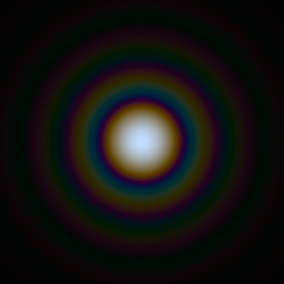
The point spread function (PSF) describes how a point-like emitter is imaged by the optical system. In incoherent imaging, the PSF is an Airy pattern whose size and shape depend on NA and wavelength. The modulation transfer function (MTF)—the magnitude of the OTF—describes how contrast at different spatial frequencies is transmitted by the system.

Attribution: Anaqreon
Several practical insights flow from PSF and MTF:
- Airy size sets the fundamental spot size: The diameter of the central Airy disk at the sensor is approximately
d_image ≈ 1.22 · λ · M_eff / NA. Sampling at the image plane with ~2–3 pixels across this diameter preserves the shape and location of point-like features and edges. - Contrast near cutoff is low: As you approach the OTF cutoff frequency, the system transmits little contrast. Even when sampled at Nyquist, the highest frequencies carry weak signal and are easily buried by noise. This is one reason some practitioners accept a slightly coarser sampling than λ/(4·NA) when practical constraints demand it.
- Aliasing is structure-dependent: If your specimen lacks features near the optical cutoff, aliasing artifacts may be less obvious even when undersampling. Conversely, periodic or fine textures can generate pronounced moiré and false detail if sampled below Nyquist.
In post-processing, deconvolution algorithms can partially restore contrast lost to the optical blur if the sampling is adequate and the PSF is known or well-estimated. However, deconvolution cannot recover spatial frequencies never sampled (beyond Nyquist) or never transmitted (beyond the OTF cutoff). Correct sampling at acquisition remains essential.
Calibrating Image Scale and Verifying Sampling in Practice
Theory guides design, but it is good practice to measure your actual image scale and verify sampling empirically. Here are common steps to ensure your pixel-to-micrometer conversion and sampling density are correct.
Measure Pixel Size in Object Space

Attribution: RIT RAJARSHI
- Use a stage micrometer or calibration slide with known feature spacing (e.g., 10 µm divisions). Focus carefully, capture an image, and measure the number of pixels spanning a known distance. Compute
p_obj = (known distance) / (pixel count). - Repeat at several field positions to check for distortion or magnification variation across the field. Most modern systems are close to telecentric in the object space, but small deviations can matter for quantitative work.
- Document the wavelength or filter set used during calibration. While magnification does not depend on wavelength, your sampling requirements do, and you should be consistent across acquisition conditions.
Compare Against Nyquist
- Given the measured
p_objand the objective NA, computeλ/(4·NA)(and optionally0.305·λ/NAfor the Rayleigh-based heuristic) under your imaging wavelength. Confirmp_objis ≤ your chosen limit. - If
p_objis larger, consider increasing magnification, moving to smaller sensor pixels, or revising acquisition settings (e.g., disabling excessive binning) to meet Nyquist.
Inspect for Aliasing
- Use fine test patterns such as high-contrast line gratings or microfabricated targets. Gradually increase spatial frequency and look for the onset of moiré or direction-dependent artifacts—these indicate undersampling.
- Rotate the specimen or camera slightly. If patterns change or move relative to the specimen detail, that is a signature of sampling-induced aliasing rather than specimen structure.
- Check edge transitions. Stair-stepping or ringing near sharp edges can be symptoms of coarse sampling and/or processing artifacts. Compare with expectations from PSF and MTF models if available.
Finally, record your calibration results, including objective, tube lens, camera model and pixel size, binning, and computed p_obj. Embedding this metadata in your workflow reduces errors and accelerates method reproducibility.
Common Pitfalls: Empty Magnification, Over- and Under-Sampling
Several recurrent misconceptions and pitfalls can degrade image quality or waste resources. Here is a concise guide to avoid them.
Empty Magnification
Empty magnification occurs when you increase magnification beyond what is required by the optics and sensor to resolve available detail. For example, if your system already satisfies Nyquist, further increasing magnification does not add resolvable information; it only spreads it over more pixels, shrinking the FOV and potentially increasing noise per pixel for a given exposure. A bit of oversampling can be helpful, but large factors rarely pay off unless you have a specific analysis goal (e.g., sub-pixel localization, PSF characterization) and adequate SNR.
Undersampling and Aliasing
Attribution: GAllegre
Undersampling (p_obj above Nyquist) risks aliasing. This can present as false periodic textures, distorted feature sizes, or inconsistent morphology that depends on object orientation. Unlike noise, aliasing is a deterministic artifact of sampling and is not easily removed after acquisition. In critical applications—quantitative morphology, metrology, or publication-quality imaging—design conservatively to avoid aliases by following the limits in Nyquist Sampling Criteria.
Ignoring Wavelength Dependence
Because resolution and Nyquist limits scale with wavelength, a setup that is Nyquist-adequate at red wavelengths may become undersampled at blue or green. If your imaging modality spans multiple bands, choose sampling based on the shortest wavelength of interest (or change sampling parameters with the filter set if your workflow allows).
Confusing Optical Resolution with Pixel Resolution
A high-resolution sensor does not guarantee high optical resolution. The optics must support the spatial frequency content, which is primarily governed by NA and system alignment. Conversely, superb optics cannot deliver their potential if the camera undersamples. Treat optics and sensor as a matched pair, linked by magnification—see Relating Sensor Pixel Size, Magnification, and Sample Scale.
Overlooking System Alignment and Stability
Focus drift, vibration, or misalignment can blur details and mimic the effect of coarse sampling by reducing high-frequency contrast. Ensure mechanical stability and appropriate focusing mechanisms. Sampling theory presumes a stable, well-corrected optical image; if the image is degraded before it reaches the sensor, meeting Nyquist will not restore lost detail.
Assuming Binning Is Always Harmful
While binning reduces sampling density, it can boost SNR and frame rate. If you designed your system with generous oversampling, moderate binning can be an effective, reversible lever to adapt to dim specimens or dynamic scenes. Just verify that the effective p_obj after binning remains below the Nyquist threshold defined in λ/(4·NA).
Frequently Asked Questions
Do I need different sampling for brightfield and fluorescence?
The sampling criterion itself—derived from NA and wavelength—does not depend on modality; it applies to incoherent imaging broadly. However, practical choices often differ. In brightfield, the image is broadband and contrast at the highest spatial frequencies may be lower, so some users choose sampling slightly coarser than the strict OTF-based Nyquist limit, accepting a small risk of aliasing in exchange for larger FOV or higher speed. In fluorescence, where emission bands are narrower and structures can be very fine, it is common to target sampling at or finer than the Nyquist limit for the relevant emission wavelength to preserve detail for deconvolution and analysis. Always recompute with the wavelength characteristic of the information you seek.
How do scanning techniques (e.g., confocal) change Nyquist?
The same Nyquist principle applies, but the PSF and OTF differ from widefield due to the confocal pinhole and scanning geometry. As a result, recommended pixel sizes in object space can differ slightly, and axial sampling rules apply for z-stacks. Nonetheless, the core idea remains: compute the system’s spatial frequency support (which depends on NA, wavelength, and modality-specific factors) and sample at least twice that frequency. For lateral sampling in confocal with typical pinhole sizes, many practitioners use spacings comparable to or slightly finer than the widefield Nyquist guideline based on λ/(4·NA). Consult the specific modality’s transfer characteristics for precise recommendations.
Final Thoughts on Matching Camera Sampling to Microscope Optics
Attribution: SiriusB
Digital microscopy works best when optics and sensor are treated as a coordinated system. The objective’s NA and the imaging wavelength set the attainable resolution and the bandwidth of spatial frequencies delivered to the camera. The camera’s pixel size, via the effective magnification, determines how finely that bandwidth is sampled. Bringing these pieces together yields a clear, actionable rule: keep the object-side pixel pitch at or below λ/(4·NA) to satisfy Nyquist across the optical passband. Where necessary, adjust magnification or choose a sensor with smaller pixels to meet this limit.
From there, optimize for your application: preserve field of view where it matters, leverage modest oversampling for robust analysis and deconvolution, and use binning judiciously when SNR or speed are limiting. Verify your configuration by calibrating image scale and testing for aliasing with known targets. Above all, avoid the traps of undersampling (which invites artifacts) and empty magnification (which inflates data without adding information).
If you found this guide useful, consider exploring more articles in our microscopy series for deeper dives into related fundamentals like PSF modeling, axial sampling in 3D imaging, and quantitative contrast. To get notified when new, practical explainers are published, subscribe to our newsletter and stay up to date with weekly microscope insights.

