Table of Contents
- What Is Numerical Aperture in Microscopy?
- How Optical Resolution Is Defined: Abbe, Rayleigh, and Practical Criteria
- Magnification, Sampling, and Digital Resolution on Sensors
- Illumination, Condenser NA, and Image Contrast
- Depth of Field, Depth of Focus, and Working Distance
- Refractive Index, Immersion Media, and Coverslips
- Optical Aberrations and Objective Corrections
- Field of View, Eyepiece Field Number, and Camera Sensors
- Modulation Transfer Function and Contrast Transfer
- Practical Alignment Principles for High-Resolution Imaging
- Frequently Asked Questions
- Final Thoughts on Optimizing Resolution and Contrast in Light Microscopy
What Is Numerical Aperture in Microscopy?
Numerical aperture (NA) is the most important single number on a microscope objective if your goal is to understand image clarity, detail, and light-gathering ability. Defined as NA = n sin θ, it combines two geometric/optical factors: the refractive index n of the medium between the specimen and the objective’s front lens, and the half-angle θ of the widest cone of light that the objective can accept or emit. In practical terms, a higher NA means the lens collects light from wider angles and supports finer spatial detail (higher spatial frequency) in the image.
It’s useful to separate what NA tells you from what magnification tells you. Magnification scales the size of the image you see or record. NA, on the other hand, sets the physical limit on the finest details that can be transferred with contrast. A common misconception is that more magnification always yields more detail. In reality, “empty magnification” spreads the same optical information over more pixels or a larger apparent size without revealing new structure. Avoiding empty magnification starts by understanding NA.

Artist: Happie1Soul
Several everyday consequences follow from NA’s definition:
- Light collection: For fluorescence and low-light imaging, higher NA objectives collect more of the emitted or transmitted light, improving signal and signal-to-noise ratio.
- Resolution: The lateral resolution limit improves (the minimum resolvable spacing gets smaller) as NA increases and as wavelength decreases. We detail the exact relationships in How Optical Resolution Is Defined: Abbe, Rayleigh, and Practical Criteria.
- Depth of field: Increasing NA decreases the axial range that appears in focus. See Depth of Field, Depth of Focus, and Working Distance for more.
- Immersion media: Switching from air (n ≈ 1.00) to water (n ≈ 1.33), glycerol (≈ 1.47), or oil (≈ 1.515) increases the achievable NA, provided the objective is designed for that medium. We discuss trade-offs in Refractive Index, Immersion Media, and Coverslips.
On specifications sheets, you will see common NA ranges such as 0.10–0.25 (low-power air objectives), 0.40–0.95 (medium to high dry objectives), and up to ≈1.4 for oil immersion objectives designed for standard cover glass. The objective’s NA is only part of the story: for transmitted-light brightfield, the condenser’s NA and illumination coherence also influence resolution and contrast. We return to that essential pairing in Illumination, Condenser NA, and Image Contrast.
Key takeaway: NA is the bridge between optics and physics in a microscope. It governs resolution, brightness, and focus thickness more directly than magnification does.
How Optical Resolution Is Defined: Abbe, Rayleigh, and Practical Criteria
“Resolution” in microscopy refers to the smallest separation at which two features can be distinguished as separate. How we quantify that depends on the sample type and illumination conditions. Classic criteria establish well-grounded limits you can use to estimate what your system can and cannot resolve.
Abbe’s periodic pattern criterion
Abbe approached resolution by considering a specimen with a periodic structure (for example, a grating). In incoherent imaging (typical of fluorescence and well-adjusted Köhler brightfield), the highest spatial frequency transmitted by the objective is proportional to 2 NA/λ, where λ is the wavelength in the specimen medium. From that, the minimum resolvable period (spacing) is approximately:
d ≈ λ / (2 · NA)
This expression is widely used to estimate achievable lateral resolution for extended structures under incoherent or partially coherent conditions close to incoherent. It tells you that halving the wavelength or doubling the NA halves the smallest resolvable spacing.
Rayleigh’s point-separation criterion
Rayleigh formulated a criterion for the resolvability of two point-like sources (or point-spread functions). In incoherent imaging, two equal-brightness point sources are considered just resolvable when the principal maximum of one overlaps with the first minimum of the other. The approximate lateral separation is:
d ≈ 0.61 · λ / NA
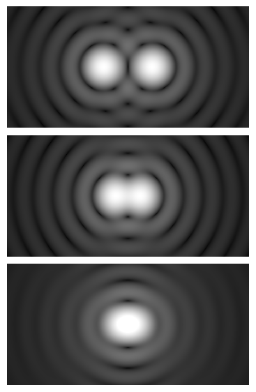
Artist: Spencer Bliven
While the numerical factor (0.61) differs from Abbe’s, both express the same dependencies: shorter wavelengths and higher NA improve resolution. Rayleigh’s form is commonly cited for point emitters (e.g., fluorescence beads), whereas Abbe’s is convenient for periodic features.
Coherence and cut-off frequency
Resolution also depends on the coherence of illumination and detection. Two useful reference points are:
- Coherent imaging (e.g., coherent laser illumination in transmission): Cut-off spatial frequency ≈ NA/λ and corresponding period
d ≈ λ/NA. - Incoherent imaging (e.g., fluorescence): Cut-off ≈ 2·NA/λ, yielding Abbe’s
d ≈ λ/(2·NA).
Most transmitted-light brightfield microscopes with properly set up Köhler illumination operate in a regime closer to incoherent than coherent, especially when the condenser aperture is opened appropriately. We discuss condenser aperture effects in Illumination, Condenser NA, and Image Contrast.
Axial resolution (sectioning) in widefield
Axial resolution (along the optical axis) is poorer than lateral resolution in widefield microscopy. A frequently cited dependence for axial resolution under incoherent conditions indicates that it scales inversely with approximately NA² and directly with wavelength. The exact expressions differ for specific imaging modalities, but the qualitative trends are robust: use shorter wavelengths and higher NA for thinner optical sections in widefield. Confocal and structured illumination techniques improve axial sectioning beyond widefield limits, but those are distinct modalities with their own criteria.
Resolution is about contrast transfer
Both Abbe’s and Rayleigh’s expressions are idealized: real optics transmit decreasing contrast at higher spatial frequencies even before the formal cut-off. That is why it is often more informative to think in terms of “usable contrast” at a given frequency rather than a single magic number. The Modulation Transfer Function (MTF) captures this idea mathematically.
Key takeaway: Regardless of which exact criterion you use, improving resolution always comes down to increasing NA and/or using shorter wavelengths, while maintaining sufficient contrast at the frequencies of interest.
Magnification, Sampling, and Digital Resolution on Sensors
Magnification is the ratio of the image size to the object size. In visual observation, total magnification is typically the product of objective magnification and eyepiece magnification. In camera-based systems, magnification is better understood as how much the specimen is “projected” onto the sensor, determined by the objective and the tube lens (in infinity-corrected systems), or by the objective and camera adapter optics.
Critically, magnification does not create detail; it scales what the optics already deliver. To capture all the available optical information digitally, your camera must sample fine enough. That’s where the Nyquist sampling principle enters.
Nyquist sampling for microscopy images
The Nyquist criterion says you need at least two samples per highest spatial frequency you wish to reconstruct. In practical microscopy terms, you should aim for a sample-plane pixel size (the pixel size at the specimen) that is about half of your optical resolution limit for unbiased capture of detail. Using the Rayleigh expression for lateral resolution r = 0.61 · λ / NA, a common digital sampling target is:
sample-plane pixel size ≤ r / 2 = 0.305 · λ / NA
Many practitioners use a slightly stricter rule of thumb (around one third of r) to provide a margin for processing and ensure robust sampling across wavelengths and field positions.
Relating camera pixel sizes to sample-plane pixel size
Let pcam be the physical camera pixel size (e.g., 3.45 µm), and Meff the effective magnification from the specimen to the sensor. Then:
sample-plane pixel size = p_cam / M_eff
For infinity-corrected objectives, Meff is the objective magnification scaled by the ratio of the actual tube lens focal length to the design tube lens focal length of the objective. For systems with camera adapters, the adapter magnification multiplies into the effective magnification. The specifics vary by system, but the principle is the same.
Example: checking sampling against optics
Suppose you image at 550 nm with a high-NA oil-immersion objective of NA = 1.40. A Rayleigh-based lateral resolution estimate is r ≈ 0.61 × 0.55 µm / 1.40 ≈ 0.24 µm. Nyquist sampling would then suggest a sample-plane pixel size of approximately ≤ 0.12 µm.
If your camera has 3.45 µm pixels and you image through an effective 60× magnification, the sample-plane pixel size is 3.45 µm / 60 ≈ 0.0575 µm. This is safely finer than 0.12 µm, meaning you are oversampling relative to the optics. Oversampling can be acceptable, though it increases data size and may not improve signal-to-noise. By contrast, if you had only 20× effective magnification, the sample-plane pixel size would be ≈ 0.1725 µm, which would undersample the optics at this wavelength and NA.
Empty magnification and visual observation
At the eyepieces, increasing magnification far beyond what your NA supports produces empty magnification: a larger, blurrier view with no new details. A practical way to think about this is to match total magnification to the resolution limit so that the smallest resolvable detail subtends a comfortable visual angle at the eye. In camera systems, the parallel is choosing optics and adapters so the pixel sampling meets or exceeds Nyquist for the optical bandwidth, but not by an extreme factor.
Spectral dependence and polychromatic imaging
Because resolution depends on wavelength, a color camera or broadband illumination implies that the effective resolution is different in each color channel. The blue channel (shorter wavelengths) often supports higher optical resolution than the red channel, all else equal. For accurate sampling, choose a pixel size that respects the shortest wavelength of interest.
Key takeaway: Proper sampling turns what the optics resolve into trustworthy digital data. Without it, you either waste information (undersampling) or inflate file sizes without gaining detail (extreme oversampling).
Illumination, Condenser NA, and Image Contrast
Resolution formulas describe what the objective could transfer in ideal conditions. Real images also depend on how the specimen is illuminated. In transmitted-light microscopy, the condenser focuses light onto the specimen and its numerical aperture plays a role analogous to the objective’s. Brightfield, darkfield, phase contrast, and differential interference contrast (DIC) each manipulate illumination differently to create or enhance contrast, but all benefit from appropriate aperture control and alignment.
Köhler illumination and partial coherence
Köhler illumination, a standard arrangement in modern microscopes, de-couples illumination uniformity from imaging focus by focusing an image of the light source at the condenser aperture and a field stop at the specimen plane. The outcome is an even field of view and well-controlled partial coherence. Partial coherence means the illumination is neither perfectly coherent (like an ideal laser) nor perfectly incoherent, but somewhere in between. This matters because image contrast and resolution depend on the balance of objective NA and condenser NA.

Images donated as part of a GLAM collaboration with Carl Zeiss Microscopy – please contact Andy Mabbett for details.
Artist: ZEISS Microscopy from Germany
Balancing condenser NA and objective NA in brightfield
In brightfield, a practical balance is to set the condenser aperture to a fraction of the objective NA. A common guideline is to open the condenser to roughly 70–90% of the objective’s NA. Opening the condenser aperture increases resolution and fine detail but can reduce phase-contrast-like edge enhancement and overall image contrast. Stopping it down increases contrast and depth of field, but can blur fine spatial frequencies and accentuate diffraction artifacts. Finding the right balance depends on your specimen’s intrinsic contrast and the details you need to emphasize.
Darkfield, phase contrast, and DIC: illumination as contrast engineering
- Darkfield blocks central rays and illuminates the specimen with oblique light so that only scattered light enters the objective. It rejects unscattered (background) light, enhancing visibility of fine scatterers at the expense of some resolution and high NA requirements.
- Phase contrast converts phase differences in transmitted light into intensity differences through specialized condenser and objective components. It raises contrast for transparent specimens but slightly compromises resolution and introduces halo artifacts near edges.
- DIC creates intensity contrast from gradients in optical path length using beam-shearing and polarizing optics. It delivers crisp, shadow-cast-like images of transparent samples with high lateral resolution, at the cost of directional shading and specific hardware requirements.
Each method has its own illumination geometry. Their influence on resolution is often subtle and tied to how coherence and pupil functions are modified. When in doubt, analyze how the method changes the effective pupil and which spatial frequencies are emphasized or suppressed. For foundational trade-offs, see the discussion of MTF and Contrast Transfer.
Depth of Field, Depth of Focus, and Working Distance
“How much of my sample looks sharp at once?” and “How forgiving is focus?” are two practical questions rooted in three related but distinct concepts: depth of field (DOF), depth of focus, and working distance.
Depth of field (specimen space)
DOF describes the axial range in the specimen within which features appear acceptably sharp. In widefield imaging, DOF shrinks rapidly as NA increases and as wavelength decreases. That’s why high-NA objectives have a very thin focus slice. Conceptually, DOF scales inversely with approximately NA² and directly with wavelength and refractive index in the specimen space. While exact formulas vary by definition of “acceptable sharpness,” the qualitative dependence is robust: higher NA yields thinner DOF.
Depth of focus (image space)
Depth of focus, by contrast, refers to how much the image plane (e.g., camera sensor position) can shift along the optical axis while the image remains acceptably sharp. It grows with magnification and is related to the f-number in photography. A system with a large depth of focus is more tolerant of small sensor placements or mechanical drift. Although depth of focus and depth of field are related, they are not the same and live on opposite sides of the objective.
Working distance (mechanical clearance)
Working distance is simply the mechanical distance from the front lens of the objective to the specimen at focus. It is a mechanical design parameter, not an image-quality metric, but it strongly correlates with NA: for a given objective class and focal length, higher NA typically comes with shorter working distance. Long working distance objectives exist for applications such as thick specimens or micro-manipulation, but they often sacrifice some NA relative to standard objectives of similar magnification.
Understanding these three together helps guide realistic expectations and setup choices. If your study demands maximum lateral resolution, you may need to accept very shallow DOF and minimal working distance. If instead you need clearance and more axial tolerance, consider a slightly lower NA objective. For additional constraints introduced by refractive index and cover glass, see Refractive Index, Immersion Media, and Coverslips.
Refractive Index, Immersion Media, and Coverslips
The refractive index of the medium between the specimen and the objective’s front element determines both the maximum achievable NA and how rays bend at interfaces. Properly matching immersion medium and cover glass is critical for preserving resolution and minimizing aberrations, especially at high NA.
Immersion media and achievable NA
- Air (n ≈ 1.00): Limits maximum NA for dry objectives. High-performance dry objectives approach NA ≈ 0.95.
- Water (n ≈ 1.33): Water immersion objectives are designed to operate with water between the front lens and the specimen or cover glass. Their NA can exceed that of comparable dry objectives and are suitable for imaging aqueous specimens to reduce refractive index mismatch in live or hydrated samples.
- Glycerol (n ≈ 1.47): Provides an index between water and oil; useful for intermediate refractive index samples or mounting media. Objectives designed for glycerol immersion maintain higher NA with reduced spherical aberration at certain depths in these media.
- Oil (n ≈ 1.515): Standard immersion oil matches the refractive index of typical cover glass. Oil-immersion objectives achieve the highest NA in common use (about 1.3–1.4) by virtue of the higher index and optimized lens design.
Coverslip thickness and spherical aberration
Most high-NA objectives are designed for a specific cover glass thickness, commonly specified as 0.17 mm (a standard associated with #1.5 cover glass) and for a certain refractive index of the glass. Deviating significantly from the design thickness or index introduces spherical aberration that reduces contrast and effective resolution, particularly off-axis and deeper into the specimen. Many high-NA objectives are very sensitive to this; even small deviations can degrade performance noticeably.
Correction collars and practical matching
Some objectives incorporate a correction collar that allows limited compensation for cover glass thickness or refractive index variations. Adjusting the collar changes the internal spacing of lens elements to reduce spherical aberration near the design value. Careful matching of immersion medium, cover glass thickness, and objective design specification is essential for leveraging the theoretical resolution limits discussed in How Optical Resolution Is Defined.
Refractive index mismatch and depth imaging
When imaging into thick specimens, especially with high NA, refractive index mismatches between immersion medium, cover glass, mounting medium, and specimen can lead to depth-dependent spherical aberration and focal shift. Water or glycerol immersion objectives can mitigate some of these effects when imaging aqueous samples. Oil immersion objectives, while reaching the highest NA near the coverslip, may suffer faster degradation in image quality as focus moves deeper into samples with mismatched indices.
Key takeaway: The closer your sample environment matches the objective’s design assumptions (immersion index, cover glass thickness), the more of the theoretical resolution you will realize in practice.
Optical Aberrations and Objective Corrections
Even with perfect alignment and matching media, lenses are subject to aberrations—departures from ideal imaging—that affect sharpness, color fidelity, and field flatness. Objective design combats these through careful choice of glass types and element shapes. Understanding objective classes helps set expectations for resolution and contrast across the field.
Common aberrations in microscopy
- Spherical aberration: Rays at different radial distances from the axis focus at different axial positions. It reduces contrast, particularly at high NA and with cover glass mismatch.
- Chromatic aberration: Different wavelengths focus at different axial positions (longitudinal chromatic) or magnify differently (lateral chromatic), causing color fringes or focus shifts across wavelengths.
- Coma and astigmatism: Off-axis aberrations that distort point images and lines, contributing to non-uniform sharpness across the field.
- Field curvature: The best focus lies on a curved surface rather than a plane, producing edges that go out of focus when the center is sharp (or vice versa).
Objective correction classes and what they imply
- Achromat: Corrected for two wavelengths (typically in the blue and red) to share a common focus and offers basic correction for spherical aberration at a reference wavelength. Often not flat across the whole field; some field curvature is expected.
- Plan Achromat: Adds field-flattening corrections so the image remains in focus across a larger portion of the field of view. Chromatic correction remains similar to achromat for two wavelengths.
- Fluorite (Semi-Apochromat): Improves chromatic and spherical correction over achromats and often provides higher NA at comparable magnifications. Designed for better transmission and fluorescence work while reducing aberrations.
- Apochromat: Offers advanced chromatic correction across three or more wavelengths with stringent control of spherical aberration. Frequently combined with plan correction (Plan Apo) for flat-field, high-NA imaging across the view.
The jump from one class to the next often yields observable gains in edge-to-edge sharpness, color consistency, and usable resolution at high spatial frequencies. However, even the best-corrected objective delivers its full potential only when paired with appropriate illumination settings, immersion media, and digital sampling.
Field of View, Eyepiece Field Number, and Camera Sensors
Resolution and contrast determine what details you can see; field of view (FOV) determines how much of the sample you see at once. In visual observation, eyepiece field number (FN) and objective magnification set the diameter of the observable field. In camera imaging, sensor size and optics control the captured area.
Eyepiece field number and visual FOV
The field number is the diameter (in millimeters) of the intermediate image the eyepiece can relay to the eye. The approximate field diameter at the specimen (visible area) is:
FOV_diameter ≈ FN / objective_magnification
For example, with FN = 20 mm and a 20× objective, the specimen-plane field diameter is roughly 1 mm. Plan-corrected objectives help keep this field sharp from center to edge. Extremely wide FNs demand objectives and tube lenses that support large intermediate images without vignetting or off-axis aberrations.
Camera sensors and relay optics
Camera-based systems replace the eyepiece with a sensor that captures the intermediate image. The diagonal and aspect ratio of the sensor, plus any intermediate lenses (tube lens and camera adapter), determine the FOV on the specimen. A larger sensor at the same effective magnification covers a wider area than a smaller sensor.
There is a trade-off between FOV and optical uniformity. As you capture wider areas, off-axis aberrations, illumination falloff, and field curvature become more prominent unless the optics are designed and aligned to support the larger field. Plan-corrected objectives and well-matched tube lenses are crucial here.
Stitching and mosaics
When a single FOV cannot cover your region of interest at the resolution you need, one approach is to acquire overlapping tiles and stitch them computationally. For accurate stitching, uniformity of magnification and illumination across the field is helpful, which circles back to Köhler illumination, stable focus, and well-corrected optics.
Modulation Transfer Function and Contrast Transfer
While resolution criteria provide a single threshold, image quality is better captured by how much contrast the system transfers at different spatial frequencies. The Modulation Transfer Function (MTF) quantifies this: it plots output contrast versus input contrast as a function of spatial frequency. The MTF is derived from the system’s Optical Transfer Function (OTF), which combines amplitude (MTF) and phase (phase transfer function).
Why MTF matters
A system with an excellent MTF sustains appreciable contrast at high spatial frequencies. Even if two objectives share the same nominal NA and thus similar cut-off frequencies, their MTFs can differ due to aberrations, coatings, and design optimizations. Thus, two lenses could have the same theoretical resolution limit but yield images with very different clarity for fine textures.
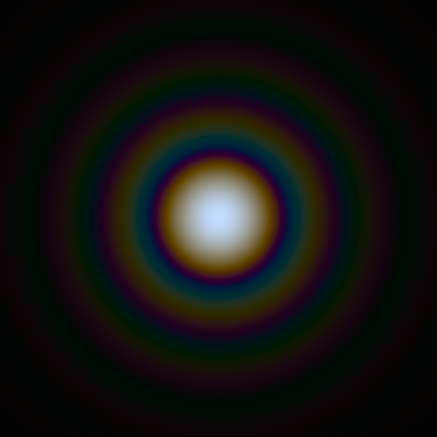
Artist: SiriusB
Qualitative behavior of MTF in microscopes
- Contrast generally decays with increasing spatial frequency, approaching zero at the cut-off frequency (which corresponds to Abbe/Rayleigh limits depending on coherence and criteria).
- Aberrations flatten the MTF curve, reducing contrast at mid to high frequencies first.
- Partial coherence and pupil modifications (e.g., phase contrast rings, DIC prisms) reshape the MTF, emphasizing certain spatial features while de-emphasizing others.
Sample, detector, and processing interactions
Apparent image sharpness depends on the interplay of the microscope’s MTF, the sample’s intrinsic spectrum of spatial features, the detector’s sampling MTF (affected by pixel size and fill factor), and any post-processing (deconvolution, denoising). Because sampling discretizes the optical image, the detector’s pixel aperture introduces an additional contrast roll-off, especially when approaching the Nyquist limit. Oversampling moderates this detector MTF loss, but with diminishing returns once you exceed the optical bandwidth significantly.
Key takeaway: Think of resolution as “contrast at the smallest details you care about.” A high NA sets a high ceiling; a strong MTF ensures you can actually see up to that ceiling.
Practical Alignment Principles for High-Resolution Imaging
High-resolution imaging relies on sound optical alignment and consistent practices. While each microscope has its own hardware and documentation, several general principles help safeguard the resolution and contrast your system is capable of delivering. The following are educational concepts rather than procedural instructions:
- Center and conjugate planes: In Köhler illumination, certain planes are conjugate with the field and aperture stops. Keeping these conjugate planes aligned preserves uniform illumination and appropriate partial coherence. See Illumination, Condenser NA, and Image Contrast.
- Objective cleanliness and immersion integrity: Dust, residue, or bubbles at the front lens reduce contrast and can scatter light, especially noticeable at high NA. Matching immersion medium to the objective design and ensuring a continuous, bubble-free interface maintains the intended pupil function. Related considerations appear in Refractive Index, Immersion Media, and Coverslips.
- Cover glass matching: Using cover glasses at the specified thickness and index (often around 0.17 mm for high-NA objectives) helps prevent spherical aberration that would otherwise degrade resolution toward the edges and with depth.
- Condenser-aperture discipline: Adjust the condenser aperture relative to the objective NA to favor the balance of resolution and contrast you need, aware that stopping down increases DOF but lowers high-frequency contrast.
- Sampling awareness: Coordinate magnification and camera pixel size so that the Nyquist criterion is met at the wavelengths and NAs you use. Avoid severe undersampling; avoid burdensome oversampling unless it serves a clear purpose (e.g., precise localization, post-processing).
- Minimize aberration sources: Mechanical tilt, mis-centering, or strain in optical elements can introduce asymmetric aberrations. Even excellent objectives benefit from square, coaxial components and a well-adjusted tube lens.
These alignment principles dovetail with the physics discussed earlier. Respecting conjugate planes, pupil functions, and sampling ensures that the theoretical limits of NA and wavelength translate into practical image quality at the camera or eyepiece.
Frequently Asked Questions
Does increasing magnification always improve resolution?
No. Resolution depends primarily on numerical aperture and wavelength. Magnification scales the size of the image but does not add detail beyond the optical information delivered by the objective and the illumination. Once you reach the point where the smallest optical details are clearly sampled and displayed, further magnification mostly makes the image larger without revealing new structure. This is called empty magnification. To ensure you are not in empty magnification territory with a camera, check that your sample-plane pixel size satisfies the Nyquist sampling target for your objective’s NA and the wavelength of interest.
Why is the condenser NA important if the objective NA sets resolution?
In transmitted-light imaging, the condenser determines how light is delivered to the specimen. Its NA and aperture influence the coherence of illumination and the angular distribution of rays that interact with the sample. If the condenser NA is set too low relative to the objective NA, high spatial frequencies may not be efficiently illuminated or transferred, reducing resolution and altering contrast. Conversely, opening the condenser aperture increases resolution potential but can lower global contrast. Balancing condenser and objective NA (often setting the condenser to about 70–90% of the objective NA in brightfield) helps achieve both adequate resolution and useful contrast. For an in-depth look, see Illumination, Condenser NA, and Image Contrast.
Final Thoughts on Optimizing Resolution and Contrast in Light Microscopy
When you strip away brand names and accessories, optical microscopy performance hinges on a tight set of interlocking principles. Numerical aperture and wavelength set the fundamental limits; illumination geometry and partial coherence determine how close you can get to those limits; aberration control, immersion matching, and cover glass conformity keep the optics operating as designed; and finally, digital sampling translates optical performance into faithful data. Misjudging any one of these can mask the gains made elsewhere.
As you evaluate or refine a microscopy setup, start with NA: choose the highest NA compatible with your specimen, immersion medium, and working distance needs. Pair it with illumination settings that promote both resolution and contrast in your modality, and make sure your camera sampling is appropriate for your wavelength and NA. If you extend FOV with larger sensors or mosaics, recognize the increased demands on flat field and off-axis correction. And as the specimen’s refractive index landscape becomes more complex or your imaging depth increases, prioritize immersion media and objectives that are designed for such conditions.
These fundamentals are not just academic. They shape everything from the crispness of a diatom’s frustule in brightfield to the localization of fluorescent puncta in a cultured cell. Apply them consistently and you will capture more of what your microscope is already capable of revealing. To continue exploring topics like Köhler illumination, objective design, and detector optimization, consider subscribing to our newsletter so you never miss future deep dives into the science and craft of microscopy.

