Table of Contents
- What Numerical Aperture and Resolution Mean in Optical Microscopy
- How Wavelength, Refractive Index, and Immersion Media Influence Detail
- Magnification: Useful vs Empty and Matching Optics to Sensors
- Depth of Field, Depth of Focus, and Working Distance Trade-offs
- Contrast, Brightness, and How NA Governs Signal-to-Noise
- Sampling, Pixel Size, and the Nyquist Criterion in Digital Microscopy
- Choosing Objectives: NA, Correction, Immersion, and Cover Glass
- Common Misconceptions About Resolution and Magnification
- Frequently Asked Questions
- Final Thoughts on Optimizing Resolution and Magnification
What Numerical Aperture and Resolution Mean in Optical Microscopy
Few topics in microscopy generate as much confusion—and as many performance gains when understood—as numerical aperture (NA), resolution, and magnification. While magnification is what most beginners first notice, resolution is what determines whether that magnified view actually reveals new detail. At the heart of resolution lies numerical aperture, a dimensionless number that quantifies the light-gathering and detail-resolving power of an objective or condenser.
Numerical aperture is defined as NA = n · sin(θ), where n is the refractive index of the immersion medium between the sample and the objective’s front lens (e.g., air, water, or oil) and θ is half the angular aperture of the objective—the maximum half-angle of light the objective can accept from the specimen. Larger NA means a wider cone of collected light and higher resolving power.
Resolution in optical microscopy is fundamentally limited by diffraction. No matter how perfect the lenses, light passing through an aperture spreads into a pattern described by diffraction theory. Two bright points that are too close together will blur into an indistinguishable spot. Several practical criteria are used to define the minimum resolvable separation. Two of the best known are:

Artist: Anaqreon
- Rayleigh criterion (lateral): approximately 0.61 · λ / NA
- Abbe limit (lateral): approximately λ / (2 · NA)
Both expressions give similar scales for the smallest lateral feature you can distinguish, with slight differences in the numerical constant due to how each criterion defines “just resolved.” In widefield brightfield microscopy, the Rayleigh criterion is a common reference point; in Fourier-based discussions, Abbe’s spatial frequency cutoff (roughly 2 · NA / λ) is often used. The key idea is consistent: shorter wavelengths and higher NA produce finer detail.
Resolution in the axial direction (along the optical axis) is more stringent. For a conventional widefield system, the axial resolution scales approximately with n · λ / NA². While the exact constants depend on imaging modality, this scaling highlights a useful design rule: increasing NA improves lateral resolution roughly linearly but improves axial resolution more strongly, roughly as the inverse square. This is one reason high-NA objectives make thin optical sections appear sharper and out-of-focus blur thinner, even in simple brightfield.
Where does magnification enter the picture? Magnification does not create new detail; it simply enlarges the image. If the optical system cannot resolve a feature, magnification will only make a blur larger. Conversely, insufficient magnification wastes optical resolution by projecting tiny details onto too few pixels (in digital imaging) or too small an image (visually). That is why one must match magnification to the sampling method and to the achievable resolution set by NA and wavelength.
A helpful mental model is to think of the microscope as a chain: illumination → objective (NA) → tube lens → camera/eyepiece (sampling) → perception/analysis. If any link mismatches the others, overall performance will be limited by the weakest link. The objective’s NA sets a physical bound on detail; magnification and sampling must be chosen to capture and convey that detail effectively.
In the sections that follow, we examine how wavelength, immersion media, and refractive index shape optical performance; how to avoid empty magnification; how depth of field interacts with NA; and how to pick objective characteristics that suit your task. Together, these ideas form the foundation of microscopic image quality for both visual and digital observation.
How Wavelength, Refractive Index, and Immersion Media Influence Detail
Because diffraction depends on wavelength, the choice of light color (or emission wavelength in fluorescence) directly influences the minimum resolvable feature. For a given NA, shorter wavelengths deliver finer resolution. For example, comparing blue light to red light can yield noticeably sharper edges and finer spatial frequencies at the same optical settings.
But wavelength is only half of the story. The other half is the refractive index of the medium between the sample and the objective’s front element. This is captured in NA’s definition, NA = n · sin(θ). If you image through air, n is approximately 1.00. With water immersion, n is on the order of 1.33. With typical microscope immersion oil, n is around 1.515 at green wavelengths. Because n multiplies the sine of the acceptance angle, moving from air to water or oil enables a higher NA for a similar geometric design, and therefore a smaller diffraction-limited spot and finer resolution.
Immersion media also reduce refraction mismatch at the sample-cover glass interface. Many biological or transparent samples are mounted under a thin coverslip. If you use a high-NA objective designed for a particular coverslip thickness and refractive index, the wavefronts entering the lens will be closer to the design condition, reducing spherical aberration and improving contrast and resolution.

Artist: Thebiologyprimer
Key points about immersion and refractive index:
- Air objectives are convenient and versatile, but their achievable NA is generally limited (typically up to roughly 0.95 in specialized designs). They minimize mess and are suitable for many applications where ultra-fine resolution is not required.
- Water immersion objectives improve resolution versus air and are helpful for aqueous samples. Water’s refractive index is closer to that of many biological media, reducing spherical aberration, especially when focusing deeper into water-rich specimens.
- Oil immersion objectives allow the highest NAs in conventional brightfield and fluorescence imaging of thin, cover-glass-mounted specimens. Oil’s refractive index is matched to standard glass, minimizing refraction at interfaces and enabling NA values exceeding 1.3.
Note that immersion choice is inseparable from specimen geometry. For thin, cover-glass-mounted samples at or near the coverslip, oil objectives excel. For thicker aqueous specimens where you wish to focus tens of micrometers deep, water immersion can outperform oil because it reduces wavefront error in the volume of interest.
In addition to lateral resolution, higher NA and refractive index matching affect axial resolution and optical sectioning. As NA increases and aberrations decrease, the point spread function becomes tighter in depth, improving contrast between in-focus planes and out-of-focus background. This benefit shows up in widefield and is particularly significant for fluorescence, where background light can overwhelm dim signals.
Finally, remember that the condenser—used in transmitted-light methods—also has an NA. To fully exploit an objective’s resolving power in brightfield or phase contrast, it helps when the condenser NA approaches or matches the objective’s NA. This ensures that the specimen is illuminated with the spatial frequencies the objective can collect. Incoherent illumination strategies like Köhler illumination are designed to make this matching practical and to achieve uniform, high-contrast lighting.
If you plan to choose or change immersion media, consider the objective’s correction and cover-glass specification, and also how your sensor sampling will respond to the increased resolution. You may reveal new detail, but only if the rest of the system is set up to capture it.
Magnification: Useful vs Empty and Matching Optics to Sensors
Magnification describes how large the microscope makes the specimen appear. With eyepieces, this is often reported as the objective’s nominal magnification multiplied by the eyepiece power. With camera-based systems, the effective magnification is the ratio between the camera’s sensor pixel pitch and the size of a pixel mapped onto the specimen plane.
However, magnification alone does not guarantee detail. If you magnify an unresolved blur, you get a larger blur. The phrase empty magnification refers to increasing magnification beyond what the optical resolution (set by NA and wavelength) and the imaging detector (set by pixel size and sampling) can support. Empty magnification does not add information; it only enlarges the same limited content.
To avoid empty magnification, you want to match magnification to both the diffraction-limited resolution and the Nyquist sampling recommended for digital acquisition. A useful rule of thumb for digital systems is:
- Ensure the object-plane pixel size (the size of one camera pixel mapped onto the specimen) is no larger than about one-half of the diffraction-limited resolution. Many practitioners target one-third (≈3 pixels across the smallest resolvable feature) to improve interpolation and deconvolution.
Mathematically, if d is the lateral diffraction-limited resolution (e.g., Rayleigh’s 0.61·λ/NA), the Nyquist condition suggests p_obj ≤ d / 2, where p_obj is the pixel size in the object plane. If your camera has pixel pitch p_sensor, and the microscope projects an overall magnification M onto the sensor, then p_obj = p_sensor / M. Rearranging, a minimum useful magnification is roughly:
M ≥ 2 · p_sensor / d
Two consequences follow:
- If you increase resolution by increasing NA or using shorter wavelengths (decreasing d), you should generally increase magnification to maintain adequate sampling.
- If your camera has very small pixels, excessive magnification is unnecessary; your pixels may already adequately sample the optical resolution at moderate M.
For visual observation through eyepieces, decades of microscope practice suggest that “useful visual magnification” typically falls within a range of roughly 500–1000× the NA of the objective. This heuristic reflects the resolving power of the human eye and the desire to make the resolution element comfortably visible. Importantly, it is a guideline, not a hard limit; visual acuity, illumination, and contrast influence practical preferences. The core message is unchanged: scale the image to suit the resolving element.
Consider these implications for camera-based imaging:
- Field of view vs. magnification: At higher magnification, you inspect smaller areas of the sample per frame. If your task requires surveying large regions, you may prefer a lower magnification objective and possibly tile images—provided sampling still satisfies Nyquist.
- Signal-to-noise: Magnification spreads the same photon budget over more pixels. If photon counts are limited, very high magnification can reduce per-pixel signal, demanding longer exposure or higher gain. The brightness and SNR trade-offs become critical here.
- Resolution-limited by optics vs. sensor: If you are under-sampling (pixels too large, magnification too low), the sensor limits your detail. If you are well-sampled but do not see new features when increasing magnification, the optics are the limit.
Bringing it all together: begin with the NA and wavelength to estimate d. Then choose magnification so that p_obj is at most half (ideally one-third) of d. This approach avoids empty magnification while ensuring you capture the fine detail your optics make available.
# Given:
#   NA = 0.85 (air), lambda = 550 nm (0.55 µm), pixel = 3.45 µm
# Rayleigh-limited resolution d ≈ 0.61 * λ / NA
lambda_um = 0.55
NA = 0.85
d = 0.61 * lambda_um / NA   # ≈ 0.61 * 0.55 / 0.85 ≈ 0.395 µm

# Nyquist: p_obj ≤ d / 2  →  p_sensor / M ≤ d / 2
# Solve for M: M ≥ 2 * p_sensor / d
p_sensor = 3.45  # µm
M_min = 2 * p_sensor / d    # ≈ 2 * 3.45 / 0.395 ≈ 17.5×

# Interpretation: an overall magnification of ~20× or higher
# would adequately sample the optical resolution on this camera.
Depth of Field, Depth of Focus, and Working Distance Trade-offs
High resolution comes with geometric consequences. As NA increases, the cone of accepted rays widens, making the system more sensitive to axial position. This is reflected in three interrelated concepts: depth of field (DOF), depth of focus, and working distance.
- Depth of field is the axial distance in the object space over which features appear acceptably sharp in the image. In widefield imaging, diffraction sets a fundamental contribution to DOF that scales on the order of n · λ / NA². As NA increases, DOF shrinks rapidly.
- Depth of focus is the permissible axial displacement at the image plane (sensor or intermediate image) while maintaining acceptable sharpness. It scales with similar dependencies but expressed in image space, often growing with magnification for a given object-side DOF.
- Working distance is the physical gap between the objective’s front lens and the specimen at focus. High-NA objectives typically have shorter working distances, especially at high magnifications, because the lens must sit close to the sample to admit a wide cone of light.
Practical outcomes:
- Focusing becomes more critical as NA rises. The system will “snap” in and out of focus over smaller axial steps. This is great for sectioning thin structures but can be challenging for thick or uneven specimens.
- Surface topography vs. volume imaging: If your sample has significant height variation, a very high-NA objective may miss relevant features that lie outside the shallow DOF. In such cases, you might step the focus and combine planes computationally (focus stacking) or select a slightly lower NA that balances resolution with DOF.
- Clearance and safety: Short working distances demand careful handling to avoid collisions. For thick samples or those with irregular surfaces, objectives with longer working distance (often with slightly lower NA for the same magnification) may be preferable.
Choosing NA is therefore not just about maximizing resolution. It is an optimization problem involving your specimen’s thickness, the structures of interest, illumination level, and how much axial discrimination you need. For thin, flat specimens, maximize NA. For thicker, uneven samples, consider the operational ease, working distance, and brightness/SNR trade-offs as you select NA.
Contrast, Brightness, and How NA Governs Signal-to-Noise
While resolution often takes center stage, contrast and signal-to-noise ratio (SNR) determine whether details are practically visible. NA influences image brightness and contrast in two ways: by affecting how much light is collected from the specimen and by shaping the point spread function that blends neighboring structures.
In epi-illumination (e.g., reflected light or fluorescence), the amount of light collected from a point in the specimen typically scales with the square of the objective’s NA. Intuitively, a wider acceptance cone captures more emitted or reflected photons per unit time, boosting signal. In transmitted brightfield, the objective’s NA also affects how much diffracted light from fine features is captured, which contributes to edge contrast.
Several practical consequences flow from these dependencies:
- Higher NA improves photon collection: All else equal, you can achieve better SNR in the same exposure time. This is especially critical in low-light methods like fluorescence. Even in brightfield, finer detail often becomes more apparent because higher spatial frequencies are transferred with higher contrast.
- Illumination NA matters in transmission: If the condenser NA is too low relative to the objective NA, the illumination may not excite the higher spatial frequencies the objective could otherwise capture. Matching or approaching objective NA with the condenser NA helps realize the objective’s resolution potential.
- Contrast mechanisms interact with NA: In phase contrast or differential interference contrast (DIC), the visibility of phase gradients and edges depends on both the optical design and the NA. Higher NA can sharpen gradients but may also reduce depth cues if the DOF becomes very thin.
Remember that SNR is not solely about photons. Electronic noise in the camera, read noise, and pattern noise can dominate at low signals. However, by raising NA—and thus photon throughput—you reduce the fractional impact of these noise sources. This is one reason that, in challenging low-light imaging, an objective with a incrementally higher NA can outperform a lower-NA lens even if nominal magnification is unchanged.
Brightness, resolution, and sampling are entangled: as you raise magnification to achieve proper sampling, you spread photons over more pixels, potentially lowering per-pixel SNR. The typical workflow is to select the NA that delivers the needed resolution and then set magnification and exposure to balance sampling and SNR for your detector.
Sampling, Pixel Size, and the Nyquist Criterion in Digital Microscopy
Digital microscopy introduces another necessary condition for sharp images: adequate sampling. Even if your optics can resolve a detail of size d, your camera must sample the image finely enough to represent that detail without aliasing. This is the essence of the Nyquist criterion.
In one dimension, the Nyquist-Shannon sampling theorem states that to represent a signal with maximum spatial frequency f_max without aliasing, you must sample at a rate exceeding 2 · f_max. In microscopy, f_max is set by the optical transfer function’s cutoff, which for incoherent imaging is on the order of 2 · NA / λ. Translating this into a real-space sampling interval yields the familiar condition that the pixel size in the object plane should be no larger than roughly half the smallest resolvable feature.
The practical procedure is:
- Estimate lateral resolution d from NA and wavelength (e.g., d ≈ 0.61 · λ / NA).
- Compute the required object-side pixel size: p_obj ≤ d / 2 (Nyquist). Target d / 3 if you plan deconvolution or fine interpolation.
- Relate object-side pixel size to sensor pixel size via magnification: p_obj = p_sensor / M. Solve for M to choose optics or relay lenses appropriately.
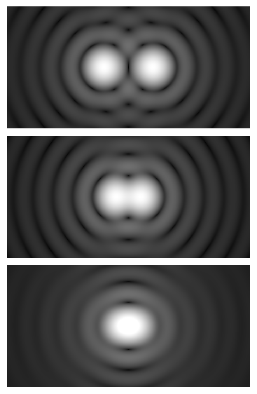
This image uses a nonlinear color scale (specifically, the fourth root) in order to better show the minima and maxima.
Artist: Spencer Bliven
Two-dimensional sampling introduces another nuance: the pattern of pixels. Most cameras use square pixels on a rectangular grid, so the 1D Nyquist condition applies similarly in both axes. Microlens arrays atop pixels in many CMOS sensors help collect more light but do not change the sampling requirement; the underlying pixel pitch sets the sampling interval.
What happens if you under-sample? High spatial frequencies (fine details) become misrepresented as lower-frequency patterns—this is aliasing. Edges can show jaggedness, and fine textures may appear as moiré. Over-sampling, on the other hand, uses more pixels than necessary to represent the optical detail. Over-sampling is generally benign (and can aid processing), but it spreads photons across more pixels, potentially lowering per-pixel SNR for a fixed photon budget.
Common pitfalls and remedies:
- Using a low-magnification objective with large-pixel sensors: You may be under-sampled and effectively limited by the camera, not the optics. Remedy: increase magnification or use a camera with smaller pixels to meet Nyquist.
- Confusing total system magnification with optical performance: A large nominal magnification may still be under-sampled if the intermediate optics de-magnify onto the sensor. Always compute object-side pixel size.
- Changing wavelength without re-evaluating sampling: If you switch from red to blue excitation/emission in fluorescence, you have improved the theoretical resolution. Consider increasing magnification to keep sampling matched to the new, smaller d.
Sampling also connects to modulation transfer function (MTF), which describes how contrast at different spatial frequencies passes from object to image. Even below the cutoff frequency, contrast tends to fall with increasing spatial frequency. Adequate sampling preserves the contrast that the optics deliver. If you under-sample, even well-transferred spatial frequencies can be misrepresented. When optimizing a system, you want the MTF of the optics and the MTF of sampling (the pixel aperture function) to work together, not against each other.
Before acquiring critical images, run a quick calculation or use a sampling calculator to ensure that p_obj meets the Nyquist condition. This simple check prevents many headaches and ensures that the resolution you paid for with high NA is actually present in your data.
Choosing Objectives: NA, Correction, Immersion, and Cover Glass
Selecting an objective is about more than magnification. Objectives differ in numerical aperture, optical corrections, immersion medium, working distance, and cover-glass specification. Each attribute influences image quality, convenience, and compatibility with your specimen and imaging method.
Numerical aperture and magnification
For a given magnification, objectives come in a range of NAs. Higher NA improves resolution and brightness but often reduces working distance and depth of field. When comparing, remember that NA is the primary driver of resolvable detail; magnification simply scales that detail to the detector or your eye. If your application demands fine lateral and axial resolution, prioritize higher NA and then ensure your magnification and sampling are appropriate.

Artist: PaulT (Gunther Tschuch)
Optical corrections
Objectives are also classified by their correction for aberrations and field flatness. Terms you may encounter include:
- Achromat: Corrected for chromatic aberration at two wavelengths and spherical aberration at one. Common and cost-effective.
- Plan (e.g., Plan Achromat): Improves field flatness so that the image is in focus across more of the field of view—useful for imaging large areas or with cameras that capture the full field.
- Apochromat: Enhanced chromatic and spherical aberration correction across more wavelengths, yielding better color fidelity and sharpness, often at higher NA and cost.
These corrections do not change the diffraction limit per se, but they make more of the field meet that limit and reduce color fringing and blur due to aberrations. For color imaging or fluorescence with multiple channels, improved chromatic correction can be particularly valuable.
Immersion medium and refractive index
As discussed in How Wavelength, Refractive Index, and Immersion Media Influence Detail, immersion choice determines the maximum practical NA and affects aberration when imaging through coverslips and media. Typical choices are:
- Air: No fluid needed. Simplest handling. Moderate to high NA possible but limited relative to immersion.
- Water: Good refractive match for aqueous samples. Useful for imaging into thicker, water-based specimens with reduced spherical aberration at depth.
- Oil: Best for highest NA at or near the coverslip for thin specimens. The refractive index of immersion oil is chosen to match standard cover glass and objective design.
Choose the immersion based on sample geometry and the structures you need to resolve. Immersion also interacts with working distance and DOF; high-NA oil lenses often have the shortest working distances.
Cover-glass thickness and correction collars
Many high-NA objectives are designed for a standard cover-glass thickness of about 0.17 mm (commonly referred to as #1.5 coverslips). If the actual cover-glass thickness or refractive index deviates from the design, spherical aberration can degrade resolution and contrast. Some objectives include a correction collar that lets you compensate for varying cover-glass thickness and, to a degree, imaging depth in a medium.

Artist: QuodScripsiScripsi
When using a correction collar, adjust it to maximize contrast and sharpness on a representative feature. Small tuning can make a visible difference, especially at high NA. If your work frequently involves nonstandard coverslips or imaging at depth, an objective with a collar can be a practical advantage.
Working distance and specimen access
If your sample has significant thickness or if you need space for micromanipulation or illumination components near the specimen, prioritize longer working distance. Objectives labeled “long working distance” (LWD) or “extra long working distance” (ELWD) trade some NA for a safer, more accessible geometry. The resolution impact is real, but workflow and specimen integrity may demand the extra clearance.
Compatibility with illumination and contrast methods
Different contrast techniques (brightfield, phase contrast, DIC, fluorescence) can require specific objective types or special internal components (e.g., phase rings, polarization properties). Ensure that the objective is suitable for your chosen method. For transmitted-light techniques, remember that achieving the objective’s theoretical resolution also depends on appropriate condenser NA and alignment.
By balancing NA, optical correction, immersion, cover-glass compatibility, and working distance, you can select an objective that delivers the resolution you need with practical usability. Always tie the choice back to magnification and sampling so that the detector captures what the optics resolve.
Common Misconceptions About Resolution and Magnification
Misunderstandings about NA, resolution, and magnification are widespread. Clearing them up can prevent wasted effort and guide smart upgrades.
“Higher magnification means better detail.”
Clarification: Magnification enlarges the image but does not create detail. Only higher NA (and shorter wavelength) reduces the diffraction-limited spot size. Magnify too far without increasing NA, and you get empty magnification.
“All 40× objectives resolve the same detail.”
Clarification: Nominal magnification does not determine resolution. A 40× objective with NA 0.65 resolves less fine detail than a 40× objective with NA 0.95. Choose by NA for resolution; use magnification to match sampling and field of view needs.
“If the image is bright, NA must be high enough.”
Clarification: Brightness can be increased with illumination power or exposure, but that does not improve resolution. NA influences both resolution and photon collection efficiency. You can have a bright yet low-resolution image if NA is limited.
“Short depth of field means the optics are flawed.”
Clarification: A shallow DOF is a consequence of high NA. It is an expected trade-off, not a defect. Use it to your advantage for thin optical sectioning, or choose a lower NA to gain more DOF when needed.
“More pixels always improve resolution.”
Clarification: If the optics limit resolution, adding pixels beyond Nyquist does not reveal more detail. Extra pixels may, however, aid interpolation, digital zoom, and noise averaging.
Frequently Asked Questions
How do I estimate the resolution I can expect from my current objective?
Start with the objective’s NA and the wavelength you use most. A common lateral estimate for widefield imaging is the Rayleigh criterion: d ≈ 0.61 · λ / NA. If you work primarily in green light (≈550 nm), plug that into the formula. For example, with NA 0.75, d is approximately 0.61 × 0.55 µm / 0.75 ≈ 0.45 µm. This is the approximate center-to-center distance of two equal-brightness point sources that are just resolved. Axial resolution is larger and scales roughly with n · λ / NA². Keep in mind that aberrations, alignment, and illumination coherence can modify practical outcomes. Once you have d, verify that your magnification and sampling are set so that p_obj ≤ d / 2.
When should I choose oil immersion vs. water immersion?
Choose oil immersion when you image thin, cover-glass-mounted specimens near the coverslip and you want the highest possible NA and lateral resolution. Oil matches the refractive index of standard cover glass and objective design, minimizing aberrations at the interface and enabling NA values above 1.3 for exceptional resolving power. Choose water immersion for thicker, aqueous specimens or when you focus deeper into a water-rich medium; the refractive-index match between water and the sample medium can reduce spherical aberration at depth, often yielding sharper images within the sample volume. In both cases, confirm that your objective is designed for the intended immersion and for the cover-glass thickness you use, and then verify that your sampling and SNR support the additional resolution you gain.
Final Thoughts on Optimizing Resolution and Magnification
In optical microscopy, numerical aperture and wavelength set the fundamental resolution; magnification and sampling determine whether you capture and perceive that detail. Higher NA reduces the diffraction limit, boosts photon collection, and tightens axial response—but it also narrows depth of field and shortens working distance. Matching magnification to the resolution element helps you avoid empty magnification and ensures your detector samples the image adequately.
As you refine your setup, use a short checklist: estimate resolution from NA and wavelength; choose immersion and objective corrections that fit your specimen and cover glass; set magnification to meet Nyquist on your camera; and balance exposure and gain for good SNR. Small, informed adjustments often yield outsized improvements in clarity and contrast.
If you found this guide useful, explore our related articles on optics fundamentals and digital imaging, and consider subscribing to our newsletter for upcoming deep dives into contrast methods, illumination strategies, and practical optimization tips for every microscopy workflow.

