Numerical Aperture, Resolution, and Depth of Field

Table of Contents

• What Do Numerical Aperture, Resolution, and Depth of Field Mean in Light Microscopy?
• How Numerical Aperture Governs Light Collection and Angular Acceptance
• Wavelength, Coherence, and the Abbe–Rayleigh Resolution Criteria
• Depth of Field vs Depth of Focus: Axial Resolution and Focus Tolerance
• Interplay of Objective NA, Magnification, and Pixel Size for Sampling
• Contrast Mechanisms and Their Effect on Apparent Resolution
• Immersion Media, Refractive Index Mismatch, and Spherical Aberration
• Practical Trade-Offs: Working Distance, Field Flatness, and Aperture Diaphragm Use
• Measurement and Calibration: Verifying Resolution in the Real World
• Frequently Asked Questions
• Final Thoughts on Choosing the Right Numerical Aperture and Resolution Strategy

What Do Numerical Aperture, Resolution, and Depth of Field Mean in Light Microscopy?

When people ask why two microscopes with the same magnification produce images of different clarity, the short answer is usually “numerical aperture.” Numerical aperture (NA) is the most important optical specification of an objective lens. It determines how much light the objective can accept and, crucially, how fine a detail it can resolve. Magnification enlarges details; NA determines whether those details exist in the first place.

To interpret microscope specifications and make sound imaging decisions, it helps to connect three pillars of image formation:

• Numerical aperture (NA): A dimensionless measure of the objective’s light-gathering and angular acceptance.
• Resolution: The smallest separation at which two features can be distinguished as distinct.
• Depth of field (DOF): The axial range in object space that appears acceptably sharp in a single focus position. Closely related is depth of focus, which is the tolerance in image space at the camera or eyepiece plane.

These concepts are linked by diffraction physics. Even a perfect, aberration-free lens cannot image arbitrarily small detail because light forms a finite-sized diffraction pattern rather than a geometric point. The size of that pattern scales with wavelength and inversely with NA, setting an ultimate limit on spatial detail. As we expand below, NA governs resolution in the focal plane, while depth of field reflects how rapidly image sharpness degrades away from focus. Increasing NA improves lateral resolution but reduces depth of field—a central trade-off that informs objective selection, sample preparation, and imaging strategy.

Before going deeper, it is useful to set terminology you will see throughout this article:

• Object space: The specimen side of the lens. Depth of field is defined here.
• Image space: The camera or eyepiece side of the lens. Depth of focus is defined here.
• PSF (point spread function): The image the system forms of an ideal point emitter. Its lateral width and axial extent underpin resolution and DOF. See Wavelength, Coherence, and the Abbe–Rayleigh Resolution Criteria.
• Condenser: In transmitted-light modes, the condenser delivers illumination to the sample with a specific angular spread, described by its own NA. This enters the resolution problem too, as covered in the resolution section and the trade-offs section.

With this foundation, we will unpack how NA is defined, how resolution depends on wavelength and illumination, why DOF shrinks with higher NA, and how sampling and contrast interplay with these limits. If you are choosing an objective or tuning a system, the guidelines in sampling and practical trade-offs will be especially helpful.

How Numerical Aperture Governs Light Collection and Angular Acceptance

Numerical aperture quantifies the range of angles over which a lens can accept or emit light. Formally, for an objective in a medium with refractive index n,

NA = n * sin(θ)

where θ is the half-angle of the largest cone of light that can enter (or exit) the lens from a point in the specimen. Two consequences follow immediately:

• Higher NA collects light from larger angles, improving both the light budget (brightness) and the system’s ability to record high spatial frequencies (fine detail).
• NA is bounded by the immersion medium. In air (n ≈ 1.0), the practical limit is NA ≲ 0.95; with water (~1.33) or oil (~1.515), NA can exceed 1.0 because n > 1. Note that sin(θ) cannot exceed 1, so increasing n is the pathway to NA > 1.

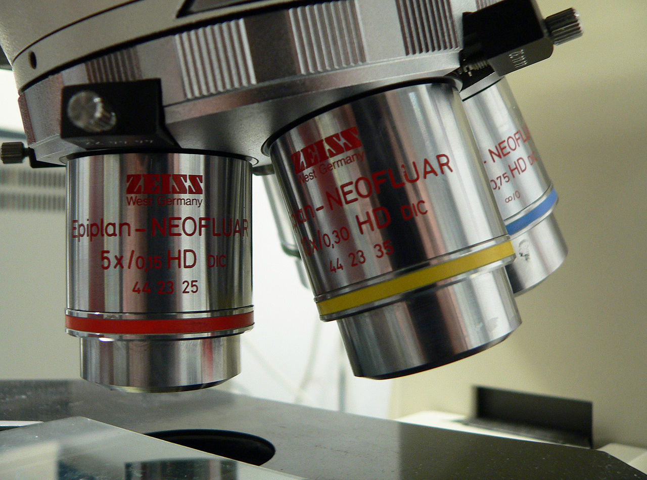
Objective markings typically list magnification and NA, for example, “40×/0.75.” In many applications, NA is a better predictor of performance than magnification. A 20×/0.8 objective may reveal more detail than a 40×/0.65 objective despite lower nominal magnification because the former captures higher-angle rays. We revisit this interplay in Interplay of Objective NA, Magnification, and Pixel Size for Sampling.

In transmitted-light imaging (brightfield, phase contrast, DIC), the condenser NA also matters because it controls the range of illuminating angles that strike the specimen. The condenser’s NA is defined similarly:

NA_condenser = n * sin(α)

with α the half-angle of the illuminating cone at the specimen. Matching condenser NA to objective NA is essential to achieve the objective’s full resolution capacity, as discussed in Practical Trade-Offs.

NA is tied to resolution through Fourier optics: a larger pupil (higher NA) passes a wider band of spatial frequencies from the specimen. The modulation transfer function (MTF) rolls off to zero at a cutoff frequency that increases with NA and decreases with wavelength. This is the frequency-domain counterpart to the well-known real-space resolution limits covered next in Wavelength, Coherence, and the Abbe–Rayleigh Resolution Criteria.

Wavelength, Coherence, and the Abbe–Rayleigh Resolution Criteria

Because light diffracts, the image of a point is not a geometric point but an Airy pattern whose bright central lobe has a finite width. Several standard criteria convert this wave-optical reality into a practical “minimum resolvable separation.” The exact numerical constants vary with definition, but the governing dependencies are the same: resolution improves (smaller numbers) with shorter wavelength and larger NA.

Rayleigh criterion for incoherent imaging

The Rayleigh criterion is often quoted for imaging of point-like features under incoherent conditions (e.g., many common widefield scenarios): two points are considered just resolved when the principal maximum of one Airy pattern coincides with the first minimum of the other. The corresponding lateral resolution in object space scales as

Δx ≈ 0.61 * λ / NA

where λ is the wavelength in the medium (or the vacuum wavelength divided by the refractive index if you explicitly account for the medium). The factor 0.61 arises from the first zero of the Bessel function governing the Airy pattern. The full-width at half maximum (FWHM) of the central lobe is smaller, often approximated as ~0.5 × λ/NA, but the Rayleigh definition provides a conservative, widely used benchmark for “just resolved.”

Abbe criterion for periodic structures

For periodic samples such as gratings, the classical Abbe theory considers which diffraction orders from the specimen are captured by the imaging system. In transmitted light with a finite-NA condenser and objective, the limiting period d is often expressed as proportional to

d ≈ λ / (NA_objective + NA_condenser)

When the condenser illuminates with a cone of angles similar to the collection cone of the objective, the sum in the denominator approaches 2 × NA, recovering the well-known “Abbe limit” in the form

d ≈ λ / (2 * NA)

Both the Rayleigh and Abbe expressions capture the same physics from different viewpoints and differ by a numerical constant because they apply to different image content (points vs periodic patterns) and different definitions of “resolved.” Importantly, the condenser aperture setting can move you between these operational regimes by altering the coherence of illumination and the effective range of illuminating angles.

Axial resolution and the 3D point spread function

Resolution is three-dimensional. The axial extent of the PSF is larger than its lateral width, producing an elongated response along the optical axis. For widefield imaging in a homogeneous medium, an often-cited scaling for the axial resolution (or axial Rayleigh criterion) is

Δz ∝ (n * λ) / (NA^2)

where n is the refractive index around the focal region. The constant of proportionality depends on the exact definition (e.g., Rayleigh-like criterion vs FWHM of the axial PSF). The key point is the inverse-square dependence on NA: doubling NA can reduce axial blur roughly by a factor of four, a powerful lever in three-dimensional imaging. The tighter axial confinement of high-NA systems comes at the cost of reduced depth of field, which is the practical range over which features appear in acceptable focus.

Rule of thumb: lateral resolution improves roughly as λ/NA; axial resolution improves roughly as λ/NA². Shorter wavelengths and higher NA help in both directions, but axial sharpness benefits even more strongly from NA increases.

Because wavelength is in the numerator, using blue light in brightfield will generally improve resolution relative to red light, all else equal. However, contrast, sample absorption, and detector sensitivity vary with wavelength, so the “shortest wavelength” is not always the most practical choice. We explore these practicalities in Contrast Mechanisms and Their Effect on Apparent Resolution.

Depth of Field vs Depth of Focus: Axial Resolution and Focus Tolerance

Depth of field (DOF) is the axial interval in object space over which features appear sharp enough for a given task. It is related to, but not identical to, axial resolution. Intuitively, DOF depends on the steepness of the PSF along the optical axis and on what you deem “acceptably sharp,” which depends on the circle of confusion set by detector sampling and viewing conditions.

Two closely related terms are easy to mix up:

• Depth of field (object space): How much you can move the specimen and still see a sharp image.
• Depth of focus (image space): How much you can move the camera/eyepiece plane (or allow defocus at the sensor) and still maintain acceptable sharpness.

For high-NA objectives, DOF is typically very small—on the order of a few micrometers or less—because the cone of focused light is very steep. This is why moving the fine focus by a tiny amount can cause dramatic changes in clarity at high NA. Qualitatively:

• DOF decreases with increasing NA (approximately with the square of NA for the diffraction-limited component).
• DOF increases with wavelength (longer wavelengths have larger DOF).
• Allowing a larger blur circle (e.g., with coarse sampling or relaxed sharpness criteria) increases DOF.

A useful conceptual model separates DOF into two additive components:

• Diffraction term: Scales approximately as (n × λ)/NA² and represents the fundamental optical blur imposed by the diffraction-limited PSF.
• Defocus tolerance term: Depends on the permitted circle of confusion, which in microscopy is closely tied to the effective pixel size at the specimen plane and the total magnification to the sensor. Finer sampling means a tighter sharpness criterion and, therefore, smaller DOF.

Depth of focus (image-space tolerance at the camera or intermediate image) expands with increasing magnification for a given NA, but because high magnification is often coupled to high NA, these relations must be considered together with sampling, covered next in Interplay of Objective NA, Magnification, and Pixel Size for Sampling.

Practically, if you need more of a thick specimen in simultaneous focus at high NA, optical sectioning or computational methods (such as focus stacking) are often used. However, those are strategies around the physics; they do not change the fundamental DOF relationship with NA and wavelength. Maintaining proper immersion and refractive index matching also helps preserve the intended DOF by minimizing aberration-induced blur.

Interplay of Objective NA, Magnification, and Pixel Size for Sampling

Even when the optics can resolve fine detail, your camera must sample the image finely enough to capture it without aliasing. The Nyquist–Shannon sampling theorem requires at least two samples across the smallest resolvable feature. In microscopy, this is often expressed as a recommended sampling of about 2–3 pixels across the width of the diffraction-limited spot (e.g., across the FWHM of the PSF’s central lobe).

The key quantities are:

• Pixel size at the sensor (e.g., 3.45 µm).
• Total magnification to the sensor (objective × intermediate optics, if any).
• Effective pixel size at the specimen:

effective_pixel_size = sensor_pixel_size / total_magnification

To satisfy Nyquist, this effective pixel size should be no larger than approximately half the lateral resolution. Using the Rayleigh-like estimate for lateral resolution, the practical guideline becomes

effective_pixel_size ≤ (0.5 to 0.33) × (0.61 * λ / NA)

The factor in parentheses reflects common practice of sampling with 2–3 pixels across the resolution element. Because the FWHM of the PSF central lobe is smaller than the Rayleigh separation, many users prefer the tighter sampling end of this range. For example, if you image with green light near 550 nm and NA = 0.8, you can compute a target effective pixel size and then choose the objective and camera magnification accordingly.

Two practical caveats:

• Avoid empty magnification. Increasing magnification without sufficient NA (or if you already sample at or beyond Nyquist) does not reveal additional detail. It only spreads the same information over more pixels.
• Consider the spectral band. If you switch illumination wavelength, the diffraction-limited spot size changes. Sampling set for green light may be too coarse for blue or too fine for red, relative to Nyquist. When imaging broadband white light, you effectively mix resolutions across the band; system MTF and detector response often favor a mid-band choice.

Sampling considerations extend into the axial dimension for 3D stacks. A rule of thumb is to step axially at roughly half the axial resolution (or finer) to satisfy Nyquist in z. Because axial resolution scales inversely with NA², high-NA imaging often requires relatively small z-steps to avoid missing axial detail.

Finally, keep in mind that contrast mechanisms influence what spatial frequencies are practically visible. High-NA optics may pass fine detail, but if the contrast of those features is low, the detector may not capture them robustly. This practical visibility is encoded in the MTF, which includes the effects of contrast, noise, and aberrations—not just the diffraction limit.

Contrast Mechanisms and Their Effect on Apparent Resolution

Resolution limits describe the smallest detail that an ideal optical system could distinguish. But whether you can see or measure that detail also depends on contrast: the difference in intensity (or phase-turned-into-intensity) between the feature and the background. Contrast mechanisms shape what parts of the specimen spectrum are emphasized or suppressed.

In transmitted-light microscopy, common contrast methods include:

• Brightfield: Relies on absorption, scattering, and refractive index variations that alter transmitted intensity. Resolution follows the standard diffraction relations, with the condenser aperture playing a major role in reaching the objective’s full NA.
• Phase contrast: Converts phase variations (optical path differences) into intensity differences using a phase ring in the condenser and a phase plate in the objective. While phase contrast can reveal structures that are nearly invisible in brightfield, it modifies the pupil function and can reduce transfer of certain spatial frequencies, slightly altering the effective MTF and apparent resolution.
• Differential interference contrast (DIC): Produces contrast from gradients in optical path length by shearing and recombining polarized beams. DIC tends to accentuate edges and slopes, improving perceived sharpness of fine features, but its transfer characteristics depend on shear, bias, and specimen anisotropy.
• Darkfield: Blocks direct (undeviated) light so that only scattered light enters the objective. This can reveal small, weakly absorbing features. Effective NA is constrained by the darkfield geometry; the illuminating cone must be larger than the collection cone, which influences resolution and signal.

These methods do not change the fundamental relationship between NA, wavelength, and diffraction-limited resolution, but they affect practical visibility of fine detail. For example, closing the condenser aperture diaphragm increases image contrast by reducing the range of illumination angles, often making low-contrast features easier to see. However, this also reduces the highest spatial frequencies admitted to the image, effectively lowering resolution. In other words, contrast adjustments can trade maximum resolution for better signal-to-noise at mid-range frequencies.

Several additional points to keep in mind:

• Wavelength dependence: Contrast in brightfield often varies by wavelength due to material absorption and scattering properties. This interacts with the λ/NA resolution scaling when choosing illumination color.
• Aberration sensitivity: Phase-based methods (phase contrast, DIC) can be more sensitive to misalignment and refractive index mismatches because they rely on controlled phase relationships across the pupil. See Immersion Media and Aberrations.
• Noise and dynamic range: Fine detail near the cutoff spatial frequency has low contrast and is susceptible to noise. Adequate exposure, detector full well capacity, and low read noise help preserve high-frequency information.

In summary, a high-NA objective sets an upper bound on resolution. Whether you can approach that bound depends on the condenser setting, alignment, sample contrast, and a host of practical factors addressed throughout this article—most notably in Practical Trade-Offs and Measurement and Calibration.

Immersion Media, Refractive Index Mismatch, and Spherical Aberration

Objectives are designed to operate in specific optical conditions. Using the correct immersion medium and cover glass thickness preserves the wavefront quality the designer assumed. When those conditions are violated, spherical aberration and other errors broaden the PSF, reducing both resolution and contrast—even if the nominal NA is high.

Immersion media and refractive index

Common immersion types include air (n ≈ 1.0), water (~1.33), and immersion oil (~1.515). The refractive index appears explicitly in the NA definition, but it also affects aberrations. When light transitions between media with different indices (specimen, cover glass, immersion layer), rays at different heights in the pupil are refracted differently. If the system is not corrected for that exact configuration, spherical aberration results, shifting best focus for marginal rays relative to paraxial rays. The observable consequences are:

• Loss of contrast, especially at high spatial frequencies.
• Broadening of the lateral and axial PSF (poorer resolution and larger effective DOF).
• Changes in apparent focus with depth in the sample, especially when imaging into thick, refractive-index-mismatched specimens.

Cover glass thickness and correction collars

High-NA objectives designed for use with a cover glass typically specify a nominal thickness (often indicated on the barrel). Deviations from the intended thickness or index cause spherical aberration. Some objectives include a correction collar that allows the user to compensate for cover glass thickness variations and specimen-induced effects within a limited range.

Practical guidance:

• Use cover glasses with thickness specifications matching the objective design. Many high-NA transmitted-light objectives assume a cover glass in a standardized thickness class.
• If present, adjust the correction collar while inspecting a fine-structure specimen to maximize contrast of the highest spatial frequencies (or to minimize the apparent halo in phase contrast). This helps null spherical aberration.
• Choose immersion media that match the intended design and the specimen environment. For aqueous specimens, water immersion can reduce index mismatch at the specimen interface relative to oil immersion, improving performance into depth, though peak NA may be lower than with oil immersion at the surface.

Imaging into depth

As you focus deeper into a specimen with refractive index different from the immersion medium, wavefront errors typically accumulate. The result is depth-dependent blur and changes in apparent axial scaling. Although the quantitative details depend on the specific indices and geometry, the qualitative lesson is robust: preserving resolution with depth requires minimizing index mismatch and maintaining the designed optical path. This dovetails with DOF considerations because aberrations effectively broaden the PSF, increasing DOF in a way that reduces true optical sectioning power.

Practical Trade-Offs: Working Distance, Field Flatness, and Aperture Diaphragm Use

Objective selection is about more than NA alone. Practicality and specimen constraints shape what is achievable. Three everyday considerations illustrate how optical specifications translate into hands-on trade-offs.

Working distance and specimen clearance

High-NA objectives gather light over a wide angular range, which typically requires a short working distance (the clearance between the objective front lens and the specimen when in focus). This can complicate imaging of thick or uneven samples. Long working distance objectives exist and can be excellent, but achieving long WD with high NA is challenging. The physical aperture needed to maintain large θ often demands a substantial front lens very close to the specimen.

Guidance:

• Assess the required clearance and sample flatness. If you need to traverse uneven topography, a moderate-NA, long-WD objective may offer a better balance of resolution and usability.
• Remember that DOF shrinks rapidly as NA rises. Even if a high-NA, short-WD lens fits, it may not accommodate the specimen’s height variation in a single frame.

Field flatness and image uniformity

Many objectives carry the descriptor “Plan,” indicating correction for field curvature so that the image is focused uniformly across the field of view. Without such correction, the edges may be out of focus when the center is sharp (or vice versa). For quantitative imaging across the whole sensor, field flatness is valuable, especially with large-format cameras.

Field flatness relates to NA and magnification because wide fields at high NA stress the lens design. Plan-corrected objectives can thus be particularly helpful when you need the edges to be as sharp as the center. This is complementary to sampling concerns because nonuniform sharpness complicates uniform sampling strategies.

Condenser aperture diaphragm and contrast vs resolution

In Köhler illumination, the condenser aperture diaphragm controls the angular spread of illuminating light at the specimen. Opening it increases condenser NA; closing it reduces NA. The setting affects both resolution and contrast:

• Open (high condenser NA): Admits high-angle illumination, maximizing resolution potential when matched to the objective NA. However, image contrast (especially for low-contrast specimens) may be lower.
• Partially closed (moderate condenser NA): Reduces the highest spatial frequencies, trading some resolution for increased contrast and depth of field. Many users find good balance with the condenser aperture set to roughly 60–80% of the objective NA.

The “optimal” diaphragm position depends on the specimen and task. When measuring fine periodic detail near the limit, open the condenser to match the objective NA. When surveying low-contrast cells or tissues where visibility of mid-frequency structure is critical, closing slightly can enhance contrast. Remember that the Abbe expression for periodic structures explicitly involves the sum of objective and condenser NA; closing the condenser reduces that sum and therefore increases the minimum resolvable period.

Tip: Use the back focal plane (accessible via a phase telescope or Bertrand lens) to visualize the overlap of the condenser pupil and the objective pupil. Matching apertures for maximum resolution, or adjusting the condenser pupil to the desired fraction for contrast, becomes straightforward.

Measurement and Calibration: Verifying Resolution in the Real World

Manufacturers specify NA and design performance under ideal conditions, but real systems include alignment tolerances, cover glass variation, and detector characteristics. Verifying practical resolution and calibrating the imaging scale helps ensure that what you interpret as “resolved” aligns with physics and with your imaging task.

Test targets and fine features

To assess lateral resolution in transmitted light, users often image patterned targets with known spacing and observe the highest spatial frequency at which lines are distinctly resolved. This checks both optical resolution and sampling together. Diatom frustules and other natural microstructures with known fine detail also serve as qualitative checks. Because the condenser aperture and illumination wavelength influence the outcome, record or control these conditions during testing.

Point spread function proxies

While true point sources are challenging in transmitted light, small scatterers can provide approximate PSFs for estimating spot size and verifying that focus and alignment yield the expected diffraction-limited width. Measuring the apparent FWHM and comparing it with the expected scaling (∝ λ/NA) is a sensitive way to detect aberrations or misalignment. If the central lobe is broader than expected across the field, revisit immersion and cover glass settings and confirm that the condenser diaphragm is set as intended.

Scale calibration

Accurate measurement requires converting pixel dimensions to object-space units. This depends on the effective magnification to the camera and any intermediate optics. Calibrate the pixel size at the specimen plane (e.g., µm per pixel) with a stage micrometer or a trusted calibration slide, under the same optical configuration used for data collection. Because the effective pixel size determines Nyquist compliance (see Interplay of Objective NA, Magnification, and Pixel Size), calibration doubles as a sampling verification.

MTF and practical contrast transfer

The modulation transfer function, if available from the manufacturer or measured on your system, provides a compact summary of contrast vs spatial frequency. While not always at hand, thinking in MTF terms can clarify why fine detail is faint even with high NA: the system may pass those frequencies with low contrast, making them susceptible to noise. Ensuring adequate illumination intensity, exposure settings, and detector dynamic range raises the practical ceiling set by noise, allowing you to approach the diffraction limit in real images.

Frequently Asked Questions

Does increasing magnification always improve resolution?

No. Magnification enlarges the image but does not create new detail. Resolution is fundamentally governed by NA and wavelength. If the optics cannot resolve a feature (e.g., because NA is too low), increasing magnification only produces a larger blurry spot. For digital imaging, increased magnification can be useful to meet Nyquist sampling requirements when you already have sufficient NA, but beyond that point additional magnification yields empty magnification without improving true resolution. See Interplay of Objective NA, Magnification, and Pixel Size for practical sampling guidance.

How should I set the condenser aperture diaphragm for best resolution?

To achieve the objective’s maximum theoretical resolution in transmitted light, set the condenser aperture so that the illuminating cone matches the objective’s collection cone (i.e., condenser NA ≈ objective NA). This ensures that the highest spatial frequencies are illuminated and collected, aligning with the Abbe criterion. However, this setting often yields lower image contrast for weakly absorbing specimens. Many practitioners close the condenser slightly—often to around 60–80% of the objective NA—to increase contrast at the cost of the very highest spatial frequencies. Choose the setting based on the specimen and whether your task prioritizes ultimate resolution or practical visibility.

Final Thoughts on Choosing the Right Numerical Aperture and Resolution Strategy

Numerical aperture, resolution, and depth of field form a tightly coupled triad in light microscopy. NA encapsulates how much of the angular spectrum your objective accepts; resolution captures how that acceptance and the wavelength translate to discernible detail; and depth of field reflects how quickly sharpness decays away from focus. The essential dependencies are consistent and powerful:

• Lateral resolution improves roughly as λ/NA.
• Axial resolution tightens roughly as λ/NA².
• Depth of field shrinks as NA rises and expands with longer wavelengths and looser sharpness criteria.

From these relationships follow practical strategies:

• Select an objective with NA appropriate for the finest detail you need to resolve, then choose magnification and camera such that you meet Nyquist sampling without drifting into empty magnification. See sampling guidance.
• Tune the condenser aperture diaphragm: match NA for maximum resolution, or close modestly to enhance contrast and ease focusing when ultimate resolution is not the immediate priority. See practical trade-offs.
• Preserve the designed wavefront by using the correct immersion medium and cover glass, and by adjusting correction collars when available. Minimizing aberration keeps the PSF tight, protecting both resolution and contrast. See immersion media and aberrations.
• Verify performance with test structures and calibrate your pixel size under the exact imaging configuration. This closes the loop between specification and reality. See measurement and calibration.

Ultimately, the “right” NA and imaging setup is the one that balances theoretical limits with specimen constraints, contrast requirements, and measurement goals. By grounding your choices in the physically correct relationships outlined here, you can extract the most from your microscope with confidence. If you enjoyed this deep dive into microscope fundamentals, consider subscribing to our newsletter to get future articles on optics, contrast methods, sampling strategies, and practical alignment tips delivered to your inbox.