Narrowband Astrophotography: Ha, OIII, SII Guide

Table of Contents

• What Is Narrowband Astrophotography and Why Use It?
• Understanding H-alpha, OIII, and SII Filters
• Choosing Cameras, Telescopes, and Mounts for Narrowband
• Planning and Framing Targets for Emission Nebulae
• Capture Workflow: Sub Exposures, Gain, and Calibration
• Processing Narrowband Data: Stacking and SHO/HOO Palettes
• Advanced Techniques: Star Reduction, Deconvolution, and Noise Control
• Common Problems and Troubleshooting in Narrowband Imaging
• Frequently Asked Questions
• Final Thoughts on Mastering Narrowband Astrophotography

Nebulae that look muted through broadband imaging can leap off the screen when captured with narrowband filters. By isolating light from specific ionized gases, narrowband astrophotography makes it possible to reveal structure and contrast—even under suburban skies and around the full Moon. This in-depth guide explains the why, what, and how: from filter physics and gear decisions to acquisition strategies and post-processing in popular workflows. Whether you shoot with a cooled monochrome camera or a one-shot color (OSC) setup using dual-band filters, you’ll find practical steps to produce striking, scientifically grounded images.

What Is Narrowband Astrophotography and Why Use It?

Narrowband astrophotography captures light in very small wavelength ranges, typically a few nanometers (nm) wide, centered on emission lines produced by ionized gases in nebulae. The three most commonly used lines are:

• Hydrogen-alpha (Hα): 656.28 nm (deep red)
• Oxygen-III (OIII): 500.7 nm (blue-green)
• Sulfur-II (SII): 672.4 nm (deep red/far red)

These lines correspond to physical processes in emission nebulae. For instance, Hα is produced when electrons recombine with protons and transition in hydrogen atoms. OIII is a forbidden transition in doubly ionized oxygen, common in high-energy regions around hot young stars, while SII traces shock fronts and lower-ionization zones. By filtering to these lines, you selectively capture gas structures while rejecting much of the broadband sky glow from urban light pollution and moonlight.

Why it matters:

• Light pollution resilience: Narrowband blocks most artificial lighting, allowing imaging from cities.
• Moon tolerance: Hα and SII are relatively robust even when the Moon is up. OIII is more sensitive to lunar brightness but still usable with careful planning.
• Contrast and structure: Filaments, shock fronts, ionization boundaries, and dust-embedded cavities appear with dramatic clarity.
• Creative color mapping: You can assign each line to color channels in various palettes, such as SHO (Hubble palette) or HOO, creating both aesthetic and scientifically meaningful renditions.

Narrowband does not replace broadband imaging for galaxies and reflection nebulae, which radiate across wider spectra. But for emission nebulae—supernova remnants, HII regions, planetary nebulae—it is a powerful approach.

You will see these concepts echoed throughout this guide, with cross-references to gear choices in Choosing Cameras, Telescopes, and Mounts for Narrowband, acquisition in Capture Workflow, and color mapping in Processing Narrowband Data.

Understanding H-alpha, OIII, and SII Filters

At the heart of narrowband imaging are optical interference filters designed to pass a tiny band of wavelengths and reject everything else. While brand names and coatings vary, the key specifications you should understand are the center wavelength, bandwidth, and transmission.

Center Wavelength and Bandwidth

The center wavelength (CWL) is the line center (e.g., 656.28 nm for Hα). The bandwidth is the width of the passband. Common bandwidths include:

• 3 nm “ultra-narrow” filters offer strong rejection of sky glow and maximize contrast but can require longer exposures and may be sensitive to bandpass shift at fast focal ratios.
• 5 nm–7 nm balances contrast and throughput, a good choice for most systems.
• 10 nm–12 nm higher throughput, easier guiding/exposure, but less suppression of sky brightness.

Transmission and Out-of-Band Rejection

High-quality filters target peak transmission often above 85–90% at the line center and steep cutoffs on either side, with strong out-of-band blocking to prevent light leaks. Effective blocking is crucial under heavy light pollution, where sodium and mercury lines (and broader LED spectra) can overwhelm weaker filters.

Fast Optics and Bandpass Shift

With fast systems (e.g., f/2–f/3), rays strike the filter at steeper angles, effectively blue-shifting the passband. Specialized “high-speed” narrowband filters compensate for this. If you use an ultra-fast astrograph, choose filters specified for your f-ratio to avoid clipping the emission line, especially in OIII and SII. For f/4–f/7 refractors and f/5–f/10 reflectors, standard filters generally perform as advertised, but verify with your manufacturer’s specifications.

Mono vs. OSC and Dual/Trio Filters

Two main imaging paths exist:

• Monochrome camera with individual filters: Highest flexibility and efficiency per line. You cycle Hα, OIII, and SII (and often Hβ for specific projects). This route is ideal for full SHO processing.
• One-shot color (OSC) camera with dual/triple-band filters: Dual-band filters typically combine Hα + OIII; some triple-band add a pass for SII or Hβ. While channel separation is less pure and signal throughput differs by CFA pattern, the workflow is simpler and faster to set up.

For a deeper system-level discussion of cameras and telescopes, see Choosing Cameras, Telescopes, and Mounts for Narrowband.

Choosing Cameras, Telescopes, and Mounts for Narrowband

Narrowband rewards careful gear selection but does not demand the most expensive setup. Matching sensor, optics, and mount performance to your seeing and goals matters more than price alone.

Cameras: Mono vs. Color, Cooling, and Pixel Scale

• Cooled mono CMOS: The gold standard for narrowband because each pixel records every photon in the chosen line. Cooling (typically down to -10°C to -20°C or lower) reduces thermal noise and stabilizes dark current.
• Cooled OSC + dual-band: Faster to operate, great for portable rigs and first steps into narrowband. Expect some crosstalk and more complex channel separation during processing.
• Pixel size and image scale: Image scale (arcsec/pixel) depends on pixel size and focal length. Aim to sample your typical seeing with approximately 1–2 arcsec/pixel; oversampling adds read noise cost without more detail, while severe undersampling makes stars blocky.

Telescopes: Refractors vs. Reflectors

• Apochromatic refractors (f/5–f/7) are popular due to tight stars, simple setup, and flat fields when used with matched flatteners/reducers. Typical apertures of 70–130 mm suit large emission nebulae and mosaics.
• Newtonian/astrographs offer larger apertures and faster optics (e.g., f/4). Collimation and coma correction are essential, but the speed helps narrowband signal.
• Catadioptrics (SCT/RC) provide longer focal lengths for small planetary nebulae or supernova remnants; however, they can be demanding on mounts and guiding.

Mounts and Guiding

• Equatorial mount: Tracks Earth’s rotation with a single axis, simplifying long exposures. Choose a mount with a realistic payload capacity above your fully loaded rig.
• Guiding and dithering: A guidescope or off-axis guider plus guiding software helps keep stars round in 3–10 minute exposures. Dithering between frames reduces fixed pattern noise and walking noise.
• Target guiding RMS: A general rule is to aim for guiding error less than half your image scale. For example, if your image scale is 2.0″/px, keep total RMS at or below about 1.0″ when possible.

Filter Wheels and Spacers

A motorized filter wheel on mono systems automates filter changes and keeps backfocus consistent. Verify backfocus spacing to your corrector or reducer within the manufacturer’s tolerance (often ±0.5–1.0 mm). For OSC dual-band filters, ensure you can place the filter at the correct optical distance to avoid tilt or vignetting.

Power and Control

Narrowband sessions often involve long exposures and all-night runs. A reliable 12V power solution with regulated outputs and a USB hub that can withstand dew and cold are practical essentials. Many imagers control rigs via mini PCs or dedicated controllers; others use laptops with planetarium and sequencing software to automate target meridian flips and filter changes.

Planning and Framing Targets for Emission Nebulae

Successful narrowband imaging starts at the desk, not the mount. Planning improves signal quality, composition, and overall efficiency.

Selecting Targets

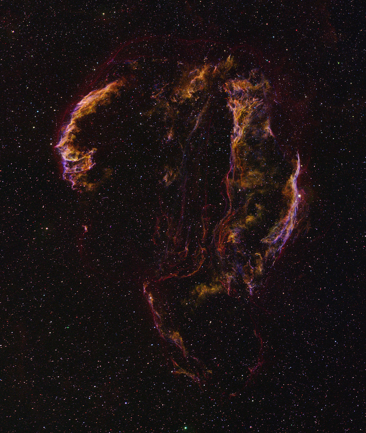
• Emission nebulae: Bright HII regions (e.g., North America Nebula), supernova remnants (e.g., the Veil), and planetary nebulae are prime narrowband targets.
• Visibility: Use planetarium software to check transit height and window of darkness. Elevation above 40–50° reduces atmospheric extinction and improves FWHM.
• Moon phase and angle: Hα and SII tolerate bright Moon phases better than OIII. If the Moon is near full, prioritize Hα, or choose targets far from the Moon’s position to minimize gradients—as discussed in Capture Workflow.

Framing and Field of View

Calculate your field of view (FOV) and image scale with your sensor and focal length. Framing tips:

• Consider a rotation angle that emphasizes shock fronts and arcs; flipping to portrait or landscape can make structures more apparent.
• Leave room for star fields or neighboring structures to avoid cramped compositions.
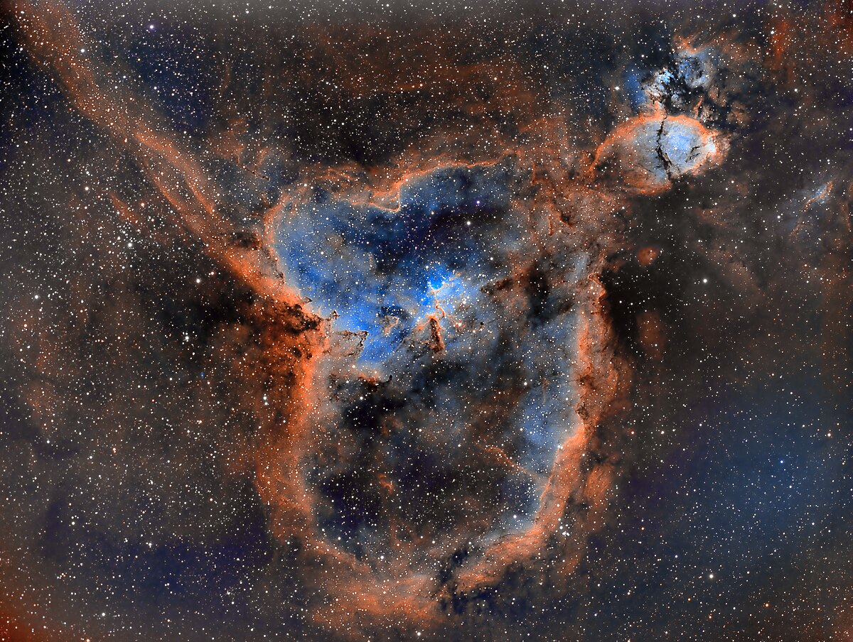
• Plan mosaics for objects like the Heart and Soul Nebulae or the Cygnus Loop; consistent overlap (10–20%) aids stitching later.

Hours per Channel

The more integration time, the better. Narrowband benefits from depth:

• For a moderate system, aim for at least 3–6 hours per channel as a starting point.
• SII is typically the faintest line; allocate extra time to SII to balance noise relative to Hα and OIII.
• If using OSC dual-band, total hours still matter—10–20 hours across multiple nights can transform the result.

Dew, Temperature, and Weather

Use dew heaters on objective lenses and secondary mirrors as insurance. Cooling your camera to a consistent set point simplifies dark calibration. When possible, choose nights with steady seeing and low wind; narrowband is less sensitive to transparency than broadband, but thin clouds still compromise star quality and flats.

Capture Workflow: Sub Exposures, Gain, and Calibration

A smooth capture workflow maximizes data quality and minimizes headaches during processing. The specifics vary by camera and software, but the core principles hold broadly.

Exposure Length and Gain/ISO

• Sub length: Typical narrowband subs range from 180 to 600 seconds. Under heavy light pollution or with bright Moon, shorter subs (e.g., 180–300s) reduce gradients. With darker skies or very narrow filters (3 nm), longer subs (300–600s) can improve efficiency.
• Gain and read noise: Many CMOS sensors have a “unity gain” region where 1 electron roughly equals 1 ADU. Operating near unity gain balances full well and read noise. Test your camera: a slight increase above unity often tames read noise without crushing dynamic range.
• Histogram check: Ensure the histogram peak is separated from the left edge—this indicates you are sky-limited rather than read-noise-limited. Narrowband histograms may look faint; don’t panic if peaks are modest.

Guiding and Dithering Strategy

• Guiding cadence: With 3–10 minute subs, 1–3 second guide exposures usually work well. Adjust aggression and hysteresis to avoid oscillations.
• Dither every few frames: Dithering every 1–3 subs helps suppress walking noise. Choose sufficient dither amplitude relative to your image scale.

Calibration Frames

Accurate calibration improves signal fidelity and makes processing easier:

• Darks: Match exposure length, temperature, and gain to your lights. Build a reusable library at common set points.
• Flats: Essential to correct vignetting and dust motes. Capture per filter and per imaging train configuration; a flat field panel or twilight sky works well.
• Bias or dark-flats: If your camera supports short exposures reliably, bias frames can model read noise. Alternatively, use dark-flats that match your flat exposure length.

Sequencing and Filter Order

• Prioritize by conditions: When the Moon is bright or high, shoot Hα and SII first; save OIII for darker windows or when the Moon is far from your target.
• Meridian flips and refocus: If your software handles flips, plan periodic autofocus, especially when temperature changes. Narrowband’s narrow passbands can shift focus more noticeably.

Tip: Build repeatable sequences for each channel, including autofocus, a short pause for settling after filter changes, and a dither after each frame or set of frames. Consistency yields cleaner stacks.

Processing Narrowband Data: Stacking and SHO/HOO Palettes

Processing is where narrowband data goes from grayscale masters to a rich, color-mapped image. Many applications can do this well—PixInsight, Siril, AstroPixelProcessor, DeepSkyStacker plus post in Photoshop or Affinity Photo. The steps are broadly similar.

Preprocessing and Stacking

1. Calibrate lights with darks, flats, and bias/dark-flats per channel.
2. Register (align) all subs across channels to a common reference. Sub-pixel registration reduces color fringing around stars later.
3. Integrate each channel separately to produce master Hα, OIII, and SII. Use pixel rejection (e.g., Winsorized Sigma Clipping) to remove satellites and artifacts.

You now have three master images: Ha, OIII, and SII. Inspect each for FWHM, roundness, and SNR. If one channel is noticeably blurrier, you can apply deconvolution or a light sharpening later, but beware of ringing near bright stars.

Linear Processing: Background and Noise

• Gradient removal: Tools such as dynamic background modeling or polynomial gradient removal can correct residual gradients, especially in OIII captured near the Moon. Perform this separately on each channel.
• Linear noise reduction: Multiscale methods can tame noise while preserving structures. Apply masks to protect bright filaments.

Channel Combination and Color Palettes

The classic combinations are:

• SHO (Hubble palette): SII → Red, Hα → Green, OIII → Blue
• HOO: Hα → Red, OIII → Green and Blue (often split or weighted)

Because Hα tends to be much stronger than SII and sometimes stronger than OIII, you may need to balance channels. Consider the following approaches:

• Scaled blending: Multiply weaker channels (SII, OIII) by gain factors or use linear fit operations before combination so that each channel contributes meaningfully.
• Dynamic narrowband mapping: Blend Hα into both the red and green channels to emphasize different structures; blend OIII into both blue and green for teal oxygen arcs.

Example pseudo-workflow (conceptual) in code-like form:


# Assume Ha, OIII, SII are calibrated, registered, linear masters
# Linear fit weaker channels to Ha for balance
OIII' = LinearFit(OIII, reference=Ha)
SII' = LinearFit(SII, reference=Ha)

# SHO combine
R = SII'
G = Ha
B = OIII'
RGB = ChannelCombine(R, G, B)

# Optional: create a synthetic luminance from Ha
L = Ha
RGB = LRGBCombine(L, RGB, lum_weight=0.6)


Nonlinear Stretching and Color Management

• Stretching: Use masked stretches or histogram transformations. Stretch gradually to protect highlights in bright cores while revealing faint tendrils.
• Color calibration: Narrowband color is not “natural”; you choose palettes for aesthetics and structure. However, star colors can be kept neutral by blending broadband stars or applying selective color adjustments after star removal.
• Green management: SHO often produces green dominance due to strong Hα in the green channel. Use color balance or green reduction tools judiciously to shift tones toward gold/blue while preserving oxygen teal hues.

Star Handling and Detail Enhancement

• Star removal: Temporarily separating stars from nebula data streamlines aggressive contrast and color work. Later, stars can be added back with controlled sizes and colors. Use star masks or star removal tools as appropriate.
• Local contrast and curves: Apply curves to boost midtones in filaments; use masks to avoid overdriving background noise.
• Deconvolution: Applied to linear luminance or Ha before stretching, deconvolution can sharpen small-scale structures. Use star masks to prevent ringing.

For techniques like star reduction and fine noise control, head to Advanced Techniques. If your result shows gradients or halos, the strategies in Common Problems and Troubleshooting can help.

Advanced Techniques: Star Reduction, Deconvolution, and Noise Control

Once your image is roughly color-balanced and stretched, advanced methods can increase clarity without artificiality.

Star Size Management

• Morphological operations: Applying a mild morphological transform with a star mask reduces star sizes. Keep iterations low to avoid doughnut stars.
• Star cores: If bright stars are bloated in OIII (common due to atmospheric dispersion or scatter), blend the star cores from Hα or a synthetic luminance to control appearance.
• Restoring star colors: Narrowband stars often lack realistic color. You can layer in stars from a short set of broadband RGB exposures if available, using screened or additive blends with careful alignment.

Deconvolution and Sharpening

• PSF estimation: Build a point spread function kernel from small unsaturated stars for deconvolution on linear data. Protect stars with masks to avoid artifacts.
• Multiscale sharpening: Wavelet- or multiscale-based contrast enhancement can boost filaments. Apply on nebula-only layers to keep stars natural.

Noise Control

• Linear noise reduction: Execute early while still linear for best results.
• Nonlinear noise reduction: After stretching, a light touch of multiscale or spatial noise reduction cleans up the background. Mask bright regions and stars.
• Dithering and stacking depth: The most effective noise reduction happens during acquisition: more total integration time and consistent dithering, as emphasized in Capture Workflow.

Starless Processing and Recomposition

Working “starless” allows aggressive stretching, selective color, and micro-contrast enhancements without bloating stars. After pushing the nebula, recombine with a lightly processed star layer at reduced opacity to keep stars tight and modest.

Common Problems and Troubleshooting in Narrowband Imaging

Narrowband solves many issues associated with broadband imaging, but it introduces its own challenges. Here are frequent problems and practical fixes.

Halos Around Bright Stars

• Cause: Internal reflections within filters or optical train, particularly in OIII where coatings and shorter wavelengths can exacerbate halo formation.
• Mitigation: Slightly refocus between filters, use filters known for low-halo coatings, minimize tilt, and ensure clean optics. In processing, star masks with halo reduction techniques can help.

Banding, Walking Noise, or Pattern Noise

• Cause: Insufficient dithering, fixed pattern noise amplified during integration.
• Mitigation: Increase dither amplitude/frequency, verify dark and bias calibration, and consider cosmetic correction in preprocessing.

Poor Star Shapes or Elongation

• Cause: Tracking errors, flexure between guidescope and main scope, wind gusts, or poor polar alignment.
• Mitigation: Improve polar alignment, use an off-axis guider to eliminate differential flexure, shorten sub exposure length if wind is strong, and ensure balanced mount axes.

Uneven Channel Sharpness

• Cause: Focus shift between filters, seeing variations over the night, or different bandpass widths.
• Mitigation: Autofocus per filter change, compensate focus offsets in software, and capture channels under comparable conditions when possible.

Gradients in OIII Under Bright Moon

• Cause: Sky brightness in the blue-green range affects OIII more than Hα/SII.
• Mitigation: Shoot OIII when the Moon is below the horizon or far from your target. Apply gradient removal during preprocessing as outlined in Processing Narrowband Data.

Color Balance and Dominant Green

• Cause: Strong Hα mapped to green channel in SHO.
• Mitigation: Use color calibration or green reduction tools and balance channels via linear fit to keep OIII/SII contributions meaningful, as described in Channel Combination and Color Palettes.

Vignetting and Dust Motes

• Cause: Filter and sensor geometry, dust on sensor window or filters.
• Mitigation: Capture accurate flats per filter and maintain a clean, sealed imaging train.

Frequently Asked Questions

Do I need a monochrome camera to do narrowband astrophotography?

No. While a monochrome camera with individual Hα, OIII, and SII filters offers the most control and efficiency per line, many imagers produce excellent results using a cooled one-shot color camera and a dual- or triple-band filter. OSC workflows simplify setup and can dramatically reduce time spent on filter changes and refocusing. The trade-off is less flexibility in channel isolation and potentially more complex channel separation during processing.

How long should I expose for each narrowband sub?

It depends on your sky brightness, f-ratio, and filter bandwidth. As a general starting point, 180–300 seconds under bright or moonlit skies and 300–600 seconds under darker conditions work well for many systems. Check that your histogram peak is off the left edge (sky-limited). If stars saturate heavily, shorten exposures or lower gain; if you are read-noise limited (histogram glued to the left), lengthen exposure or raise gain moderately.

Final Thoughts on Mastering Narrowband Astrophotography

Narrowband astrophotography opens a unique window onto the physics of nebulae, letting you trace ionization fronts, shock waves, and cavities sculpted by stellar winds and supernovae. By isolating Hα at 656.28 nm, OIII at 500.7 nm, and SII at 672.4 nm, you can reveal structure and contrast even from light-polluted sites and during the bright phases of the Moon. The keys to success are straightforward but require discipline: balanced integration time across channels, meticulous calibration, routine dithering, and thoughtful processing with masks and multiscale tools.

Start with practical goals: choose a well-placed emission nebula, plan your framing, and capture a solid baseline—say, 3–6 hours of Hα and at least as much total time across OIII and SII. Then, iterate: refine guiding and focus, try different color palettes like SHO or HOO, and experiment with starless workflows and gentle star reduction to keep attention on filaments. Over time, your portfolio will reflect both technical growth and an evolving aesthetic.

If this deep dive helped you, explore our related guides on capture strategies and post-processing. To keep up with new techniques, gear tests, and target ideas throughout the observing season, subscribe to our newsletter and never miss the next article.