Table of Contents
- What Is Signal-to-Noise Ratio in Deep-Sky Astrophotography?
- The Physics of Photons, Noise, and Modern Detectors
- Where Noise Comes From in Deep-Sky Imaging
- How to Measure and Calculate SNR in Practice
- Exposure Strategy: Subexposures, Gain/ISO, and Total Time
- Stacking, Dithering, and Calibration Frames for High SNR
- Post-Processing Choices That Preserve and Reveal SNR
- Field Workflow: Planning and Execution for Better SNR
- Frequently Asked Questions
- Final Thoughts on Maximizing SNR in Deep‑Sky Images
What Is Signal-to-Noise Ratio in Deep-Sky Astrophotography?
Signal-to-noise ratio (SNR) is the most important quantitative concept in deep-sky astrophotography. It determines whether faint galactic cirrus appears as real nebulosity or vanishes in a snowy background, whether dust lanes in a spiral galaxy are crisp or muddled, and whether star colors look natural or blotchy. Simply put, SNR compares the strength of your astronomical signal to the fluctuations that obscure it.
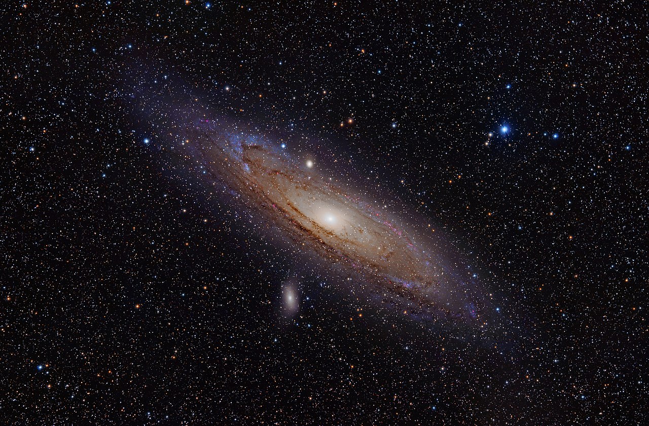
Attribution: Adam Evans
In astrophotography, the “signal” is the number of photoelectrons generated by your target (galaxy, nebula, star cluster) recorded by the sensor. The “noise” is the inherent randomness—primarily photon shot noise from the target and skyglow—plus electronics and thermal contributions. A higher SNR means you can stretch, sharpen, and color-balance with confidence; a lower SNR forces aggressive noise reduction and robs detail.
Why is SNR so fundamental compared with, say, resolution or dynamic range? Because most deep-sky scenes are photon-starved. Under a dark sky, only a trickle of photons per pixel per second reach the detector from a dim nebula. This makes the random nullgrainnull of the image—not your lens sharpness—the rate-limiting factor for quality. Boosting SNR therefore underpins nearly every decision you make in acquisition and processing, from exposure lengths to stacking to calibration strategies. Throughout this guide, we will link specific choices back to SNR so you can make decisions that are both consistent and evidence-based. For example, when we discuss exposure strategy and stacking, younullll see how those choices mathematically raise SNR, not just subjectively improve appearance.
Before we dive into methods, letnulls establish a working definition. For a single exposure, a common expression for SNR per pixel (or per aperture if you sum pixels) is:
SNR_single = S / sqrt(S + B + D + RN^2)
where:
- S = signal electrons from the astronomical target
- B = electrons from sky background (light pollution, airglow, moonlight)
- D = electrons from dark current (thermal)
- RN = read noise (electronic) in electrons
For a stack of N equal subexposures that are properly calibrated and combined, the SNR scales as:
SNR_stack ≈ sqrt(N) * S / sqrt(S + B + D + RN^2)
Equivalently, in a background-limited regime (when B dominates, which is common for deep-sky under most skies with sufficiently long subs), SNR ∝ sqrt(total integration time). This square-root law is why experienced imagers say: Hours matter. Double your total exposure time and you improve SNR by about 1.41×. The math may be simple, but it leads to powerful planning decisions younullll revisit in field workflow.
The Physics of Photons, Noise, and Modern Detectors

Attribution: NASA/Amanda Diller
Understanding SNR starts with photon statistics and how sensors collect light. Astronomical light arrives as discrete photons following Poisson statistics. If a pixel collects N photons (converted to electrons with some quantum efficiency), the intrinsic shot noise in that count is sqrt(N). There is no way around shot noise—you can only reduce its impact by collecting more photons (increasing N). This is the foundation of the square-root law that pervades astrophotography.
Digital camera sensors convert photons to electrons and ultimately to digital numbers (ADU, or analog-to-digital units). Key sensor parameters influencing SNR include:
- Quantum efficiency (QE): Fraction of photons converted to electrons. Higher QE yields more signal per unit time.
- Full well capacity (FWC): Maximum electron charge a pixel can hold before saturating. Larger FWC supports higher dynamic range.
- Read noise (RN): Random variation introduced during pixel readout and digitization, measured in electrons RMS. Lower RN makes short exposures more efficient.
- Dark current: Thermally generated electrons that accumulate even in the absence of light; suppressed by cooling.
- System gain: The conversion factor between electrons and ADU (e/ADU). With known gain, you can convert measurements in your image to electrons and compute SNR directly.
- Bit depth: Precision of the analog-to-digital converter (e.g., 12-bit, 14-bit, 16-bit). Higher bit depth reduces quantization error and preserves subtle tonal variations, but it is not a substitute for higher SNR.
Modern dedicated astronomy CMOS cameras typically feature low read noise and relatively high QE, often making them effective across a range of subexposure lengths. DSLRs and mirrorless cameras, especially when used at moderate ISO settings and in raw mode, can also deliver excellent results. However, their performance may vary with temperature and internal processing. In either case, SNR fundamentals apply regardless of the brand or the sensor: collect enough signal so that random noise sources are small compared to your astronomical signal.
A few clarifications that are often misunderstood:
- Shot noise is signal-dependent. Brighter things have higher shot noise, but they also have higher SNR because the signal grows faster than the noise (linearly vs square root).
- Read noise is independent of signal and typically constant per exposure. This is why very short subs can be inefficient when read noise is not swamped by background.
- Dynamic range is not the same as SNR. Dynamic range concerns how much brightness range you can record without clipping shadows or highlights; SNR is about how cleanly you can see detail at a given brightness level. You need both, and choices like gain/ISO affect each differently, as discussed in exposure strategy.
Where Noise Comes From in Deep-Sky Imaging
To improve SNR, you must know your adversaries. Here are the principal noise sources and confounding artifacts you will encounter:
Photon (shot) noise
Target shot noise: Your subjectnullthe galaxy, nebula, or clusternullarrives as sparse photons. If a pixel collects S electrons from the target, its shot noise is sqrt(S). The SNR contribution of the target signal alone would be S / sqrt(S) = sqrt(S).
Sky background shot noise: Skyglow (light pollution, airglow) contributes B electrons, with shot noise sqrt(B). This is often the dominant noise in calibrated frames, particularly under suburban skies or in bright lunar conditions. It limits how faint you can go and is the reason narrowband filters and dark sites are powerful SNR tools.
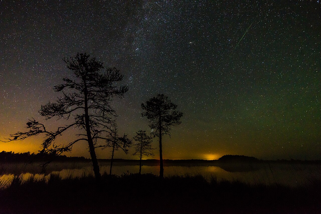
Attribution: Martin Mark
Read noise
Each exposure incurs an electronic penalty, RN. This is added in quadrature with photon noise. Short subexposures taken in large numbers can stack to high SNR, but only once read noise is a small fraction of the total noise budget. See optimal subexposure strategy for how to ensure you are background-limited.
Dark current and thermal noise
Thermally generated electrons accrue during the exposure. The rate depends strongly on temperature. Cooled astronomy cameras reduce dark current and stabilize calibration; uncooled cameras benefit from shorter exposures and careful dark/bias management to keep thermal variations under control.
Fixed-pattern noise (FPN) and amp glow
FPN appears as repeatable structure: column patterns, top-to-bottom banding, or corner brightening known as amp glow. Calibration frames and dithering are the antidotes; see stacking and calibration. FPN is not purely random, so it doesnnullt average down with stacking in the same way random noise does.
Quantization noise
Digitizing an analog signal introduces rounding errors. With reasonable bit depth and adequate signal levels, quantization noise is usually negligible compared to shot and read noise. If your subexposures place the histogram very close to the bias level, quantization error may become more apparent; adjust gain/ISO or subexposure length accordingly.
Optical and tracking effects that masquerade as noise
- Atmospheric seeing and scintillation: Blur and short-timescale fluctuations alter star shapes and intensity. They reduce effective resolution more than they change per-pixel SNR, but they complicate deconvolution and fine detail extraction.
- Guiding/tracking errors: Not random noise, but trailing smears detail and spreads signal over more pixels, reducing local SNR. Accurate polar alignment, guiding, and periodic error correction help maintain compact PSFs.
- Light pollution gradients: Slow-varying gradients can lower SNR in faint structures by elevating local background. Gradient removal during processing improves perceived SNR but can also reveal the limits of the data if overdone.
How to Measure and Calculate SNR in Practice
Theory meets the field when you can measure SNR in your data. You can do this rigorously (in electrons) if your cameranulls gain is known, or approximately in ADU if not.
From ADU to electrons
Most acquisition or processing tools can estimate or accept your cameranulls system gain (e/ADU) and read noise (enullB9 RMS). With those, you can convert pixel statistics to electrons:
- Subtract a master bias (or use bias-subtracted, calibrated frames) to remove offset.
- Measure the mean and standard deviation in a region of interest (ROI) on a calibrated light frame: one small ROI on target signal, another on blank sky background.
- Convert means from ADU to electrons by multiplying by gain:
e⁻ = ADU * gain(e⁻/ADU).
Then, using S as the target electrons above background and B as the sky electrons, estimate:
SNR_single ≈ S / sqrt(S + B + D + RN^2)
If dark current is negligible or your dark calibration is excellent, you can omit D. For stacked data, multiply the numerator by N and include N under the square root appropriately:
SNR_stack ≈ N*S / sqrt(N*(S + B + D) + N*RN^2) = sqrt(N) * S / sqrt(S + B + D + RN^2)
This formulation exposes two practical levers: increasing S (more signal via longer total exposure, faster optics, higher QE, darker skies) and controlling the denominator (reducing sky B via filters and site choice, minimizing RN with appropriate subexposures).
Practical SNR checks without full sensor characterization
Even if you do not know your exact gain, a few robust checks guide you:
- Histogram placement: In a raw linear subexposure, the sky background peak should be clearly to the right of the bias/black point. That ensures you are not starved near quantization and that read noise is swamped by sky noise. How far right depends on your camera and conditions; see exposure strategy.
- Background standard deviation: Measure the standard deviation (σ) of a star-free region. If small changes in subexposure length barely reduce σ, you are background-limited already; longer subs wonnullt help per-frame SNR much, though more total time will.
- Stacking SNR test: Stack 1, 2, 4, 8 subs and measure SNR on a fixed ROI. If SNR improves roughly as
sqrt(N), read noise and FPN are well-managed. If not, revisit dithering and calibration.
Per-pixel versus aperture SNR
Per-pixel SNR can look discouragingly low because faint structures span multiple pixels. Summing signal over a small aperture (e.g., a few pixels matching the PSF size) improves SNR as signal adds linearly but random noise adds in quadrature. Many photometric SNR formulas use aperture sums; for image quality, what matters is the effective SNR after your typical stretch and deconvolution, which benefits from both good per-pixel SNR and compact stars.
Exposure Strategy: Subexposures, Gain/ISO, and Total Time
Exposure planning is where SNR optimizations turn into concrete settings. Your goals:
- Make each subexposure background-limited rather than read-noise-limited.
- Avoid saturating bright stars or the core of galaxies more than necessary.
- Accumulate enough total integration time to reach your target SNR for faint structures.
Choosing subexposure length
A practical heuristic is to expose long enough that the sky background noise dominates read noise. In equations, you want:
Variance_sky ≫ RN^2, or equivalently,B ≫ RN^2(in electrons).
Since B = sky_rate * t, a rule of thumb is:
t_min ≈ k * RN^2 / sky_rate
where k is a safety factor (often chosen in the 5–10 range) and sky_rate is electrons per second per pixel from sky background. This is not a strict law; itnulls a planning tool. If you lack the exact rates, rely on the histogram placement heuristic: set exposure so the sky peak sits comfortably above the bias/left edge in your raw histogram. Under darker skies, t_min grows; under brighter skies, shorter subs can suffice (though total time requirements may increase due to a higher B).

Attribution: Aomorikuma
Longer subs are not always better. They risk:
- Highlight clipping: Burned-out star cores or galaxy nuclei reduce dynamic range.
- Guiding sensitivity: Wind gusts or mount periodic error can ruin longer frames.
- Satellite trails/aircraft: More time at risk per subexposure; robust rejection can mitigate but is not perfect.
In many modern CMOS workflows, moderately short exposures (e.g., dozens to hundreds of seconds for broadband, longer for narrowband) strike a good balance: they swamp read noise, retain highlights, and invite robust outlier rejection. The exact values vary with focal ratio, pixel size, sky brightness, and filter bandpass. For very narrowband filters, sky rates are tiny; longer subs are often necessary to avoid quantization and read-noise inefficiency.
Gain and ISO selection
On dedicated astro CMOS cameras, gain adjusts the conversion between electrons and ADU. A higher gain lowers the electrons-per-ADU, generally reducing effective read noise in ADU but also lowering the saturation point (reducing dynamic range). Some cameras have a nullunifiednull or nullunitynull gain where 1 electron corresponds to 1 ADU; this is often a practical midpoint, but itnulls not a universal rule. Choose gain to balance dynamic range and read-noise suppression given your target and sky.
On DSLRs and mirrorless cameras, ISO is an analog and/or digital amplification setting applied before raw encoding. Some modern sensors are close to ISO invariant over a range, meaning you can keep ISO lower to maximize dynamic range and lift shadows in processing without significant SNR penalty. However, very low ISOs can increase the impact of read noise, and very high ISOs can clip highlights and compress tonal range. A moderate ISO that keeps the background well above bias while protecting highlights is usually effective; the exact value varies by sensor generation and sky brightness.
Total integration time
Regardless of subexposure length, total time dominates final SNR once you are background-limited. Practically:
- If your SNR is too low on faint filaments after 2 hours, expect only a modest improvement with 1 more hour. To double SNR, you need roughly 4× the total exposure time.
- Diminishing returns are real but predictable; use them to plan multi-night integrations for difficult targets. See field workflow for strategies.
Broadband vs narrowband
Under heavy light pollution or bright moon, narrowband filters (e.g., HnullB1 and OnullB3 bandpasses) can produce dramatically higher SNR on emission nebulae by rejecting much of the sky background while passing key emission lines. However, stars and continuum targets (galaxies, reflection nebulae) do not benefit the same way, and the reduced passband means you need longer subs or more total time to achieve good SNR. Dual- and tri-band filters for one-shot color cameras offer a middle path for emission targets.
Stacking, Dithering, and Calibration Frames for High SNR
Well-acquired data still needs scrupulous preparation to unlock SNR. Calibration and stacking are not bureaucratic steps; they are SNR multipliers.

It is a panoramic view of the neighboring Andromeda galaxy, located 2.5 million light-years away. It took over 10 years to make this vast and colorful portrait of the galaxy, requiring over 600 Hubble overlapping snapshots that were challenging to stitch together. The galaxy is so close to us, that in angular size it is six times the apparent diameter of the full Moon, and can be seen with the unaided eye. For Hubble’s pinpoint view, that’s a lot of celestial real estate to cover. This stunning, colorful mosaic captures the glow of 200 million stars. That’s still a fraction of Andromeda’s population. And the stars are spread across about 2.5 billion pixels. The detailed look at the resolved stars will help astronomers piece together the galaxy’s past history that includes mergers with smaller satellite galaxies.
Attribution: NASA, ESA, Benjamin F. Williams (UWashington), Zhuo Chen (UWashington), L. Clifton Johnson (Northwestern); Image Processing: Joseph DePasquale (STScI)
Light frames
Your primary data: many calibrated subexposures. Strive for consistent focus, framing, and guiding. If seeing degrades or focus drifts, consider excluding poorer frames or weighting your stack to favor the sharpest subs.
Bias (or offset) frames
Very short exposures taken with the shutter closed to capture the cameranulls electronic offset and high-frequency pattern noise. With some modern CMOS sensors, bias frames behave differently from longer darks; dark flats (short dark frames matching flat exposure length) are often recommended instead of traditional bias. The goal is to model and remove the electronic pedestal and fixed patterns.
Dark frames
Exposures with the shutter closed at the same temperature, gain/ISO, and exposure time as your lights. They capture dark current and amp glow. Subtracting a high-quality master dark can eliminate structured thermal signatures, protecting SNR by reducing coherent artifacts that do not average down by stacking alone.
Flat frames
Illuminated frames that map vignetting and dust motes. Flats are critical for SNR because uneven illumination forces aggressive gradients and masking later, which exacerbates noise. High-quality flats normalize the field so that stacking and stretching reveal real signal rather than optical blemishes.
Dithering
Dithering is the practice of shifting the telescope a few pixels between subs. It breaks up fixed-pattern noise and nullwalking noisenull (banding that crawls across stacks when using drizzle or poor calibration). By moving the sky relative to the sensor grid, you convert some systematic effects into random-like noise that averaging can suppress. If you see residual banding or mottling after stacking, increase dither amplitude or frequency. This simple technique can produce a visible jump in SNR after integration.
Rejection algorithms and weighting
When stacking:
- Robust rejection (e.g., sigma clipping, Winsorized sigma) removes outliers such as cosmic rays, satellite trails, and transient gradients, protecting SNR by preserving only signal-consistent data.
- Weighting frames by FWHM, eccentricity, background level, and SNR metrics prioritizes cleaner subs, raising the effective SNR of the stack.
- Drizzle can improve sampling for undersampled data at the cost of increased apparent noise; it is most effective with large dither offsets and many subs. Use it when your pixel scale is coarser than your seeing-limited resolution and you have the data volume to support it.
Post-Processing Choices That Preserve and Reveal SNR
Processing cannot create signal where none exists, but it can preserve the SNR you captured and make it more apparent. The following practices reduce the risk of sacrificing SNR in pursuit of visual pop.
Work in the linear stage thoughtfully
Before any non-linear stretch, apply calibration verification, cosmetic correction, gradient modeling, and color calibration. Remaining in the linear domain allows noise statistics to stay well-behaved, making tools like background neutralization and noise evaluation more reliable. Stretching too early amplifies noise and complicates rejection of residual artifacts.
Gradient removal with restraint
Models such as polynomial background extraction can remove large-scale gradients that suppress local SNR. However, aggressive modeling can subtract real IFN (integrated flux nebula) or faint halos. Use star masks and well-chosen sample points; verify that structures are astrophysical (cross-check with deeper surveys if needed) before removing them as nullgradient.null
Noise reduction: luminance versus chrominance
Apply noise reduction selectively and in stages:
- Chrominance noise (color speckle) often tolerates more smoothing without destroying detail.
- Luminance noise reduction should be masked to protect high-SNR edges and small-scale structures.
- Multi-scale transforms, wavelets, and edge-aware algorithms work effectively when driven by a noise model estimated from background regions.
Remember, the best noise reduction is more photons; use it to polish, not to rescue fundamentally low-SNR data. If you find yourself battling orange-peel textures after stretching, revisit dithering and calibration or plan for more integration time.
Stretching for perceived SNR
Histogram transformations and midtone stretches can increase perceived contrast in faint structures but also raise background noise. Techniques like masked stretch and generalized hyperbolic stretch can protect highlights while lifting shadows. Combine with range masks to ensure that low-SNR areas do not dominate the visual impression with noise granularity. Iterative small stretches often outperform one aggressive move.
Star management and deconvolution
Stars are high-SNR features but can dominate the image, making faint nebulae look noisier by contrast. Star masks, morphological transforms, and star-reduction strategies can rebalance attention onto diffuse structures. Deconvolution can restore some resolution lost to seeing and optics, boosting effective local SNR by concentrating signal into fewer pixels, but it requires accurate PSF estimation and conservative regularization to avoid amplifying noise.
Color calibration and saturation
Accurate color calibration prevents hue noise from masquerading as detail. Once calibrated, moderate saturation paired with chroma noise control often yields a cleaner result than heavy saturation, which can accentuate low-SNR color blotches. For emission nebulae, narrowband combinations (e.g., HnullB1/OnullB3 blends) should be composited with attention to channel-specific SNR; stretching low-SNR channels more softly can keep the balance natural.
Field Workflow: Planning and Execution for Better SNR
Even with perfect theory, SNR gains can slip away in the field without a robust workflow. The following steps form an end-to-end plan to protect SNR from setup through packing up.
Site and timing choices
- Darkness matters: A darker site lowers
B, the background term in your noise equation, effectively increasing contrast on faint targets. If you can travel, stack the deck in your favor. - Moon phase and angle: Even narrowband imaging benefits from keeping the Moon well-separated from your target. For broadband galaxies and clusters, plan around new moon and avoid low-altitude targets where extinction and skyglow are strongest.
- Transparency and seeing: Thin clouds raise background and scatter; poor seeing spreads signal, reducing local SNR. Give marginal nights to star clusters or brighter nebulae; save very faint dust for pristine conditions.
Optical train hygiene
- Flat-field discipline: Take flats whenever you change your optical configuration (filters, focus, camera rotation). Good flats preserve SNR by preventing vignetting and dust from forcing aggressive processing later.
- Backfocus and tilt: Uneven star shapes spread signal and degrade local SNR; shimming and tilt adjustment make a measurable difference, especially with fast optics.
- Dew control: Moisture softens stars and dims the target, both SNR hits. Use dew heaters and shields proactively.
Focusing, guiding, and framing
- Refocus with temperature changes: As the night cools, focus drifts. A quick autofocus between filter changes or every degree or two preserves sharpness and SNR.
- Guiding cadence: Balance exposure time of the guide camera against mount response and seeing. Over-correcting to seeing can add jitter; under-correcting allows drift. The goal is compact PSFs that concentrate signal.
- Framing for gradients: Avoid bright sources just out of frame that produce reflections or gradients. Keeping the background smooth simplifies gradient modeling and protects faint detail SNR later.
Exposure and dither cadence
Set subexposure length using the principles in exposure strategy. Dither every few frames at minimum; for under-sampled or drizzle-intended data, dither every frame if practical. If guiding recovers quickly, a slightly more frequent dither pays for itself in cleaner stacks.
Calibration frame strategy on the same night
- Dark management: For cooled cameras, maintain consistent setpoints and build a dark library. For uncooled cameras, take darks close in temperature to your lights or rely on robust dark optimization techniques if your software supports it.
- Flats each session: Illumination patterns can change with dust and rotation. Capture new flats to prevent low-frequency noise from masquerading as structure after stretching.
Data triage and quality control
Inspect subs as the session proceeds. Reject for clouds, large FWHM spikes, wind shake, or severe gradients from passing lights. Early rejection protects SNR in the final integration by keeping the noise model consistent and the PSF compact.
Frequently Asked Questions
How many hours do I need on a target for good SNR?
It depends on your sky brightness, optics speed, filter choice, and the targetnulls surface brightness. Because SNR ∝ sqrt(total time) once you are background-limited, every 4× increase in total integration roughly doubles SNR. Under dark skies with a fast system, 3–6 hours can yield high-quality broadband images of mid-brightness targets. Very faint dust may require 10–20+ hours. Under brighter skies, you will likely need more time or narrowband filters to reach similar SNR on emission nebulae.
Does stacking many short exposures equal one long exposure?
When each short exposure is sufficiently background-limited and properly calibrated and dithered, stacking many short exposures can closely match the SNR of fewer longer exposures with the same total time. However, if subexposures are so short that read noise is a large fraction of the noise budget, they are inefficient. Also, very short subs may clip fewer highlights (good) but increase storage and processing overhead and can make rejection of outliers more complicated. A balanced approachnullshort enough to avoid clipping and handle guiding, long enough to swamp read noisenullusually wins.
Final Thoughts on Maximizing SNR in Deep‑Sky Images
In deep-sky astrophotography, everything points back to SNR. The physics says shot noise rules; the camera adds read and thermal terms; the sky sets the background. Your job is to shape this landscape so that faint astronomical signal stands out. Choose subexposures that are background-limited without sacrificing highlights. Stack generously, dither frequently, and calibrate meticulously. Process with a light touch that preserves structure and color rather than drowning low-SNR areas in aggressive stretches or denoise artifacts.
If you remember only three takeaways, make them these:
- Total integration time is king: Once you are background-limited, every extra hour improves SNR predictably.
- Control the denominator: Lower the background with site selection and filters, reduce electronics noise with appropriate gain and calibration, and break up patterns with dithering.
- Protect signal at every step: Accurate focus and guiding, high-quality flats, thoughtful stretching, and targeted noise reduction preserve the SNR you worked hard to collect.
Armed with these principles, you can plan sessions with confidence and evaluate results quantitatively. If you found this guide useful, explore our related deep-sky imaging articles, and consider subscribing to our newsletter for future installments on advanced calibration, color management, and multi-night integration planning.

This Spitzer’s 24-micron mosaic is the sharpest image ever taken of the dust in another spiral galaxy. This is possible because Andromeda is a close neighbor to the Milky Way at a mere 2.5 million light-years away.
The Spitzer multiband imaging photometer’s 24-micron detector recorded 11,000 separate snapshots to create this new comprehensive picture. Asymmetrical features are seen in the prominent ring of star formation. The ring appears to be split into two pieces, forming the hole to the lower right. These features may have been caused by interactions with satellite galaxies around Andromeda as they plunge through its disk.
Spitzer also reveals delicate tracings of spiral arms within this ring that reach into the very center of the galaxy. One sees a scattering of stars within Andromeda, but only select stars that are wrapped in envelopes of dust light up at infrared wavelengths.
This is a dramatic contrast to the traditional view at visible wavelengths, which shows the starlight instead of the dust. The center of the galaxy in this view is dominated by a large bulge that overwhelms the inner spirals seen in dust. The dust lanes are faintly visible in places, but only where they can be seen in silhouette against background stars.
The data were taken on August 25, 2004, the one-year anniversary of the launch of the space telescope. The observations have been transformed into this remarkable gift from Spitzer — the most detailed infrared image of the spectacular galaxy to date.
Attribution: NASA/JPL-Caltech/K. Gordon (University of Arizona)