Variable Stars: Types, Physics, and How to Observe

Table of Contents

• What Are Variable Stars and Why They Matter in Modern Astronomy
• A Practical Taxonomy: Intrinsic vs. Extrinsic Variable Stars
• Inside the Physics of Stellar Variability
• How Astronomers Measure Stellar Brightness and Color
• Light Curves, Period Analysis, and What They Reveal
• Using Variable Stars to Measure Cosmic Distances
• Surveys, Space Telescopes, and the Era of Time-Domain Astronomy
• How to Observe Variable Stars: Naked Eye to CCD
• From Raw Images to Science: Data Reduction and Citizen Science
• Common Pitfalls, Systematics, and Best Practices
• Frequently Asked Questions
• Final Thoughts on Exploring Variable Stars

What Are Variable Stars and Why They Matter in Modern Astronomy

Variable stars are stars whose observed brightness changes over time. These changes, recorded in a time series called a light curve, can unfold over minutes, days, or years and may be periodic, semi-regular, or irregular. Variability arises from intrinsic changes in the star itself—such as pulsations or eruptions—or from extrinsic effects like eclipses by a companion star. Far from being mere curiosities, variable stars underpin crucial measurements in astrophysics, including the scale of our universe and the life cycles of stars.

Early observers noticed stars that appeared to “wink” or shift in brightness. The eclipsing binary Algol was documented as varying by ancient astronomers and later explained in the 18th century. In the early 20th century, Henrietta Swan Leavitt’s work on Cepheid variables uncovered a tight link between pulsation period and luminosity, a relation that has since anchored the cosmic distance ladder. Today, the study of variable stars sits at the heart of time-domain astronomy, a field that focuses on how astronomical objects change with time.

Understanding variable stars serves multiple purposes:

• They reveal stellar interiors through pulsation modes and frequencies, offering asteroseismic insights into mass, radius, and age.
• They calibrate extragalactic distances via standard candles such as Cepheids and RR Lyrae, connecting nearby and faraway distance scales.
• They flag binary systems and mass transfer processes (e.g., cataclysmic variables), informing how stars evolve in pairs.
• They trace galactic structure—RR Lyrae mark old stellar populations, while Cepheids pinpoint young, star-forming regions.
• They enable citizen science, as observers of all experience levels can contribute high-value measurements, sometimes from a backyard telescope.

In what follows, we map out the rich taxonomy of variable stars, delve into the physics that power their changes, and provide practical guidance for observing and analyzing these dynamic suns. When a concept builds on earlier ideas, we’ll reference other sections via helpful internal links, such as the discussion of the period–luminosity relation in Using Variable Stars to Measure Cosmic Distances and observational advice in How to Observe Variable Stars.

A Practical Taxonomy: Intrinsic vs. Extrinsic Variable Stars

The most useful first division is between intrinsic and extrinsic variability:

Intrinsic Variables

For intrinsic variables, the star’s own properties change with time—its radius, temperature, surface features, or the stability of its outer layers.

• Pulsating Variables
  • Classical Cepheids (Population I): Young, massive stars (typically 3–12 solar masses) with periods from about 1 to ~100 days. Their pulsations are driven by an opacity mechanism and follow a strong period–luminosity relation (see distance markers).
  • Type II Cepheids (Population II): Older, lower-mass pulsators with different period–luminosity calibrations than classical Cepheids.
  • RR Lyrae: Horizontal-branch stars, lower mass than Cepheids, with short periods (~0.2–1 day). Standard candles primarily for old stellar populations like globular clusters.
  • Mira variables: Long-period variables (hundreds of days), typically cool, evolved asymptotic giant branch (AGB) stars with large amplitude changes—often more than several magnitudes in the visual band.
  • Delta Scuti and SX Phoenicis: Short-period pulsators (hours) in the instability strip, sometimes showing multiple pulsation modes.
  • RRc/RRab/RRd subtypes: RR Lyrae sub-classes indicating different pulsation modes (first overtone, fundamental, double-mode).
• Eruptive and Cataclysmic Variables
  • Flare stars: Often M dwarfs with strong magnetic activity, producing short, intense brightening events.
  • Cataclysmic variables (CVs): Close binaries with a white dwarf accreting from a companion. Includes dwarf novae (disk instability outbursts) and classical novae (thermonuclear runaways on the white dwarf surface).
  • Young Stellar Objects (YSOs) such as T Tauri stars: Variability related to accretion, starspots, and circumstellar material.
• Rotational Variables
  • Spotted stars: Rotational modulation as starspots rotate into and out of view, analogous to sunspots but often larger and more numerous.
  • Ellipsoidal variables: Tidal distortion in close binaries creates a non-spherical shape, leading to brightness modulation with orbital phase even without eclipses.

Extrinsic Variables

Extrinsic variability arises from geometry and intervening material rather than internal changes in luminosity.

• Eclipsing Binaries
  • Algol-type: Detached binaries with distinct eclipses as one star passes in front of the other. Algol itself is a textbook example.
    

    

  • Beta Lyrae-type: Semi-detached systems with continuous light variation due to a deformed, mass-transferring star.
  • W Ursae Majoris-type: Contact binaries with stars sharing a common envelope, often showing smooth, nearly sinusoidal light curves.
• Transiting Objects
  • Exoplanet transits: A planet passing in front of a star causes a small, periodic dip in brightness. Although not a traditional “variable star” class, the observed phenomenon is extrinsic variability and the light-curve analysis is similar to that for eclipsing binaries.
  • Occultations by circumstellar material: Dust clouds or disks can intermittently block starlight, especially in YSOs, leading to irregular dips.

These categories are not mutually exclusive. For example, a star can be both a pulsator and a member of an eclipsing binary. Classifications are tools for organizing phenomena, but nature often blends them. For a deeper dive into mechanisms that power each category, see Inside the Physics of Stellar Variability.

Inside the Physics of Stellar Variability

At the heart of variability lie changes in energy transport, geometry, or surface conditions. Here are the major physical drivers:

The Opacity (κ) Mechanism in Pulsators

In Cepheids and RR Lyrae, pulsations are sustained by the opacity mechanism, often called the κ-mechanism. Partial ionization zones—especially those involving helium—play a pivotal role. When the star’s outer layers compress, the opacity in these zones rises, temporarily trapping heat and raising pressure. This push drives expansion. As the layer expands, it cools, recombination occurs, and opacity drops, allowing radiation to escape and the layer to fall back. The repeating cycle sets up stable pulsations.

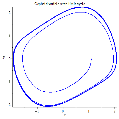
Key features include:

• Driving zone: Typically the partial ionization of helium (He I and He II) in Cepheids and RR Lyrae.
• Mode selection: Stars can pulsate in the fundamental mode, overtones, or multiple modes simultaneously—observable as characteristic shapes and harmonic content in the light curve.
• Period scaling: The period links to the star’s mean density via the classical pulsation relation; larger, less dense stars pulsate more slowly.

Convection and Large-Amplitude Pulsations

Mira variables are cool, extended AGB stars with deep convective envelopes. Their long periods (hundreds of days) and large amplitudes reflect fundamental-mode pulsations in very extended atmospheres. While the κ-mechanism still contributes, convection complicates the energy transport and light-curve shapes. Dust formation in their winds can also modulate visible light output, often smoothing or skewing maxima and minima.

Magnetic Activity and Starspots

Surface inhomogeneities—spots and faculae—cause brightness modulation tied to the stellar rotation period. Younger, rapidly rotating stars tend to be more magnetically active and thus more variable. Over longer timescales, stellar activity cycles (akin to the Sun’s approximately 11-year cycle) can change the amplitude and baseline brightness.

Binary Interactions: Eclipses, Tides, and Accretion

In close binaries, tides distort stellar shapes, creating ellipsoidal variations. In mass-transferring binaries, light curves also record the state of the accretion disk. Cataclysmic variables exhibit outbursts driven by disk instabilities: the disk alternates between low and high viscosity states, suddenly brightening when mass accretion surges. In novae, the accreted hydrogen layer undergoes a thermonuclear runaway on the white dwarf surface, resulting in a dramatic but non-destructive brightening; the white dwarf survives the event.

Dust, Disks, and Irregular Dimming

Young stars with protoplanetary disks often show irregular dimming events as clumps of dust cross our line of sight. This circumstellar extinction can change on timescales from hours to months. The phenomenon illustrates how variable stars can be probes of not just stellar physics but also the architecture of environments like disks and outflows.

Each mechanism leaves signatures in the light curve and spectrum. To recognize them, astronomers rely on precise measurements of brightness and color, explained in How Astronomers Measure Stellar Brightness and Color, and on mathematical tools for analyzing periodicity, discussed in Light Curves, Period Analysis, and What They Reveal.

How Astronomers Measure Stellar Brightness and Color

Apparent brightness is quantified in magnitudes, a logarithmic scale where a difference of 5 magnitudes corresponds to a factor of 100 in flux. Lower (more negative) magnitudes mean brighter sources. Typical measurements record a star’s flux through a specific filter bandpass—for example, Johnson-Cousins B, V, R_c, I_c, or Sloan u, g, r, i, z. Color indices (e.g., B–V, g–r) indicate temperature and, combined with models, surface gravity and metallicity.

Differential Photometry

A common observing strategy is differential photometry, where the target’s brightness is compared to nearby non-variable comparison stars in the same image. This mitigates effects of atmospheric transparency fluctuations and instrument drift.

• Pick at least one reliable comparison star and ideally a check star of similar color and brightness to the target.
• Measure instrumental fluxes (e.g., via aperture photometry) and form magnitude differences like m(target) - m(comp).
• Use catalogs with calibrated magnitudes for the comparison stars to transform to a standard system when needed.

Tip: Matching the color of the comparison and target stars reduces the impact of varying atmospheric extinction across wavelengths.

Photometric Systems and Transformations

Professional and advanced amateur work often aims to transform instrumental magnitudes to a standard system. This requires observing standard fields across a range of airmasses and colors to solve for transformation coefficients and extinction terms. For science that depends primarily on relative changes (e.g., period determination), consistent instrumental photometry can still be highly valuable without full transformation.

Signal-to-Noise Considerations

To detect millimagnitude-level variations (e.g., shallow exoplanet transits), you need high signal-to-noise ratio (SNR) and meticulous systematics control. For large-amplitude variables like Miras, lower SNR can still capture the essential features of the light curve. Exposure times must balance avoiding saturation with minimizing scintillation and read noise. Strategies are elaborated in How to Observe Variable Stars and the cautionary notes in Common Pitfalls, Systematics, and Best Practices.

Color and Temperature Changes

In pulsating stars, brightness and color changes are often phase-dependent. Cepheids tend to be bluer (hotter) near maximum light and redder (cooler) near minimum. Recording multi-band photometry reveals this thermal cycle and helps distinguish between competing physical models.

Light Curves, Period Analysis, and What They Reveal

The light curve is the central observational product in variable star astronomy: brightness versus time. From it, astronomers infer periodicities, amplitudes, shapes, and long-term trends.

Period Detection

When your data are unevenly sampled—a common reality in ground-based observing—methods like the Lomb–Scargle periodogram excel at detecting periodicities. For eclipsing binaries and pulsators with nearly sinusoidal variations, Fourier analysis and harmonic fitting are standard techniques.

• Phase Folding: Once a period is identified, plotting brightness against phase (time modulo period) reveals a repeating pattern and reduces scatter from multiple cycles.
  

  

• Harmonics: Non-sinusoidal shapes (e.g., sawtooth-like Cepheid light curves) appear as strong power at the fundamental frequency plus harmonics.
• Multi-Periodicity: Some stars exhibit multiple independent modes (e.g., Delta Scuti), requiring multi-frequency fits.

Morphology and Physical Clues

Light-curve morphology helps classify variability:

• Cepheids: Asymmetric light curves with steep rise and gradual decline; amplitude and Fourier parameters correlate with period.
• RR Lyrae: RRab types show asymmetric curves with sharp rises; RRc are more sinusoidal with smaller amplitudes.
• Eclipsing binaries: Characteristic primary and secondary minima; relative depth reveals temperature ratio and surface brightness contrast.
• Rotational modulation: Quasi-sinusoidal with evolving amplitude as spots grow and decay.
• Cataclysmic variables: Quiescent flickering plus large, episodic outbursts; superhumps can appear in SU UMa-type systems.

Timing Analysis and O–C Diagrams

Precision timing of, say, eclipse minima or pulsation maxima yields an observed-minus-calculated (O–C) diagram. Deviations from a constant period can signal mass transfer, magnetic activity cycles, light-travel time effects from additional bodies, or evolutionary changes in the star’s structure.

Spectroscopy and Radial Velocities

Photometry captures brightness changes, but spectroscopy adds velocity and temperature information. Radial velocity curves in eclipsing binaries, combined with photometric light curves, allow precise stellar mass and radius determinations. In pulsators, spectral line shifts track the breathing motions of the photosphere, complementing the light-curve phase information.

For an application that impacts cosmology, continue to Using Variable Stars to Measure Cosmic Distances. For data acquisition tactics, jump to How to Observe Variable Stars.

Using Variable Stars to Measure Cosmic Distances

Variable stars have long served as standard candles—objects with known luminosity—enabling distances to be inferred from their apparent brightness. Two classes are especially important:

The Period–Luminosity Relation (Leavitt Law) for Cepheids

Henrietta Swan Leavitt discovered that Cepheids in the Small Magellanic Cloud displayed a tight correlation: brighter Cepheids have longer pulsation periods. Because the stars in that galaxy lie at roughly the same distance, intrinsic luminosity variations could be isolated from the observed magnitudes. This period–luminosity (P–L) relation, refined over decades, is a cornerstone of the distance ladder.

• Calibration: Nearby Cepheids with geometric distances (e.g., from parallax) set the zero-point. Calibrations can be performed in optical and near-infrared bands, with the latter less affected by dust extinction.
  

  

• Metallicity Effects: The P–L relation depends on chemical composition; careful analyses account for metallicity when applying the relation to different stellar populations.
• Applications: Cepheid distances anchor the luminosity calibration of Type Ia supernovae, which probe the expansion of the universe to far larger scales.

RR Lyrae as Standard Candles of Old Populations

RR Lyrae stars have relatively uniform absolute magnitudes, especially in certain passbands, making them reliable distance indicators for globular clusters and the stellar halo of the Milky Way. Because they are older, lower-mass stars, their presence traces ancient stellar populations and galactic structure.

Mira Variables in the Infrared

Mira variables also show period–luminosity relations, particularly tight at near-infrared wavelengths where dust obscuration is reduced. Their high luminosity makes them useful for probing distances in the nearby universe, complementing Cepheids and RR Lyrae.

Building the Distance Ladder

Distances in astronomy are often determined hierarchically. Geometric methods like trigonometric parallax calibrate nearby standard candles (e.g., Cepheids), which in turn calibrate more distant candles (e.g., Type Ia SNe). Variable stars thus provide the key rung between local and cosmological scales. This connectivity is one reason why precise photometry and careful treatment of systematics (see Common Pitfalls) are so crucial.

Surveys, Space Telescopes, and the Era of Time-Domain Astronomy

Modern surveys have revolutionized variable star discovery and characterization. Dedicated space and ground-based facilities now monitor the sky with high cadence and precision, producing vast light-curve databases across multiple filters.

Ground-Based Surveys

• OGLE (Optical Gravitational Lensing Experiment): A long-running project that, among other achievements, has cataloged enormous numbers of pulsating stars and eclipsing binaries in the Magellanic Clouds and the Galactic bulge.
• ASAS-SN (All-Sky Automated Survey for SuperNovae): Despite the name, it monitors the entire sky for variability, discovering and characterizing variable stars and transients.
• Catalina Surveys and similar programs: Time-domain projects that contribute significantly to variable star catalogs, including cataclysmic variables and eclipsing binaries.

Space-Based Missions

• Kepler/K2: Provided ultra-precise, continuous light curves for hundreds of thousands of stars, revealing fine-grained variability, oscillations, and exoplanet transits.
• TESS (Transiting Exoplanet Survey Satellite): Monitors nearly the entire sky, enabling the detection of short-period variables and eclipsing binaries in bright, nearby stars.
• Gaia: Although best known for astrometry, Gaia’s photometry and variability classifications have transformed our understanding of variable star populations across the Galaxy.

These surveys not only uncover new variables but also provide homogeneous datasets for statistical studies. For instance, they map the instability strip occupancy, investigate metallicity effects on P–L relations across environments, and discover rare variable types. The flood of data makes robust analysis techniques, described in Light Curves, Period Analysis, and What They Reveal, more important than ever.

How to Observe Variable Stars: Naked Eye to CCD

Observing variable stars is accessible at all levels. You can start with naked-eye estimates of bright, high-amplitude variables and graduate to CCD or CMOS photometry capable of millimagnitude precision. The choice of technique depends on your goals and equipment.

Naked-Eye and Binocular Observing

• Mira variables like Mira (Omicron Ceti) and Betelgeuse (Alpha Orionis) make excellent targets due to their large amplitude and brightness.
• Use comparison stars of known magnitudes to estimate the variable’s brightness. Practiced observers can achieve ~0.1–0.2 magnitude precision.
• Record the date, time, sky conditions, and your estimate. Over months, your log will trace the star’s cycle.

DSLR and Mirrorless Cameras

• On a fixed tripod, short exposures can capture bright variables. For fainter targets, a tracking mount keeps stars sharp in longer exposures.
• Shoot RAW to preserve linearity; avoid in-camera processing like noise reduction that can compromise photometry.
• Calibrate with dark, bias, and (if practical) flat frames. Even modest calibration reduces gradients and improves precision.

Dedicated CCD/CMOS Photometry

• Telescope Aperture: A small telescope (e.g., 80–200 mm aperture) can reach many targets with sufficient SNR. Faster optics (lower f/number) reduce exposure time.
• Filters: Photometric filters (Johnson-Cousins or Sloan) standardize observations. V band is a common starting point; adding R_c or I_c extends temperature sensitivity and reduces extinction effects.
• Exposure Control: Avoid saturation; use multiple shorter exposures to improve SNR via averaging while preserving dynamic range.

Target Selection and Planning

• Choose targets suiting your cadence and magnitude limits. For example, RR Lyrae require minute-to-hour sampling, while Miras can be sampled weekly.
• Consider elevation and airmass. Observing near the meridian minimizes atmospheric extinction and seeing variability.
• Include a check star to validate that your comparison star is stable.

For next steps in processing, including aperture choices and transformations, see From Raw Images to Science.

From Raw Images to Science: Data Reduction and Citizen Science

Turning raw images into a calibrated light curve involves several steps. While professional pipelines automate much of this, backyard astronomers can follow a similar workflow tailored to their gear.

Calibration Frames

• Bias frames: Zero-length exposures to capture the camera’s readout pattern.
• Dark frames: Exposures at the same temperature and duration as your lights to map thermal noise.
• Flat fields: Images of a uniformly illuminated field to correct pixel-to-pixel sensitivity variations and vignetting.

Apply these to your light frames to produce clean, calibrated images. If your camera supports temperature regulation, maintain a stable sensor temperature for reproducible darks.

Aperture Photometry and Choices

Aperture photometry sums pixel values in a circular aperture centered on the star, subtracting the local background measured in an annulus. Aperture radius trades off between capturing total flux and adding noise from sky background. A typical strategy is a radius of ~2–3 times the full width at half maximum (FWHM) of the star’s point spread function. If seeing varies throughout the night, consider adjusting aperture size accordingly or using software that adapts to FWHM.

Time Stamps and Barycentric Corrections

Accurate timing is crucial for period studies, eclipses, and coordinated campaigns. Record mid-exposure times, ideally converted to a standard such as Barycentric Julian Date (BJD), which corrects for the Earth’s motion around the Sun. Consistent time standards ensure your data can be merged with others’.

Differential Light Curves and Error Bars

Construct differential magnitudes versus time: m_var - m_comp. Include uncertainty estimates, combining photon noise, sky background, and instrumental read noise. Plotting the variable minus comparison and check minus comparison helps identify issues with the comparison star or systematics in the data.

Transformations to a Standard System

To compare with published work or feed models requiring standardized colors, derive transformation coefficients by observing standard star fields. You can then convert your instrumental measurements (e.g., v, r) into standard magnitudes (e.g., V, R_c) using linear relations that include color terms and extinction.

Quality Control and Data Sharing

Adopt a consistent file naming scheme, keep a detailed observing log, and note any anomalies (clouds, guiding glitches). Many observers contribute their measurements to established databases and campaigns—coordinated data over long baselines are invaluable for trends and period changes. For considerations about avoiding common traps, jump to Common Pitfalls, Systematics, and Best Practices.

Common Pitfalls, Systematics, and Best Practices

Even simple setups can deliver scientifically useful results if you avoid systematic errors. Here are frequent hazards and how to mitigate them:

Atmospheric Effects

• Extinction: Air mass increases at lower altitudes, dimming stars and reddening their light. Observe near culmination and match target/comparison colors.
• Scintillation: Rapid twinkling imposes high-frequency noise. Longer exposures and larger apertures reduce its impact.
• Thin clouds: Can introduce time-correlated trends. Differential photometry with nearby stars helps, but clouds that vary across the field can still bias results.

Instrumental Challenges

• Saturation and non-linearity: Keep counts below the camera’s linear regime threshold; consult your detector’s specifications.
• Flat-field errors: Dust motes and vignetting change over time; update flats regularly and keep optics clean.
• Shutter timing: For very short exposures, mechanical shutter transit times can produce gradients. Electronic shutters mitigate this, but verify with tests.

Comparison Star Selection

• Avoid subtly variable comparison stars, which can corrupt your light curve. A check star helps flag this issue.
• Choose comparisons of similar color and brightness to limit color-dependent extinction differences.
• Verify catalog values and note the photometric system (e.g., V vs. g). Transform if needed.

Sampling and Alias Problems

• Cadence: Undersampling can miss sharp eclipse features or pulsation peaks. Match cadence to expected variability timescales.
• Window function: Nightly gaps create alias peaks in periodograms. Multi-longitude coordination reduces aliases and improves period accuracy.

Data Analysis Discipline

• Keep raw data and all intermediate steps reproducible. Document software, versions, and settings.
• Assess residuals after fitting. Structured residuals can signal missing physics (e.g., an additional pulsation mode) or systematics.
• Report uncertainties realistically, including both random and systematic components when possible.

Following these practices elevates your dataset from a casual record to a robust scientific measurement—one that can inform studies like period changes in pulsators or eclipse timing variations, topics explored in Light Curves, Period Analysis.

Frequently Asked Questions

How can I tell if a star is intrinsically variable or part of an eclipsing system?

Examine the light-curve shape and, if available, spectroscopy. Eclipsing binaries typically show discrete minima corresponding to primary and secondary eclipses, often with flat or gently varying maxima between them. The depths and durations of the minima are tied to the stars’ sizes, temperatures, and orbit geometry. Pulsators like Cepheids and RR Lyrae exhibit smooth, often asymmetric variations with characteristic rise and fall times, and their color and temperature change over the cycle. Radial velocity measurements can clinch the case: eclipsing binaries show orbital Doppler shifts; pulsators show velocities in phase with radius changes rather than orbital motion. Additional clues come from phase stability and harmonic content in periodograms.

What exposure time should I use for CCD photometry of an RR Lyrae?

Balance SNR against time resolution. An RR Lyrae’s period is typically 0.2–1 day with rapid changes near maximum light. Aim for individual exposures that keep peak counts below saturation while achieving sufficient SNR (often many thousands of electrons for millimagnitude precision). For a modest telescope and a bright RR Lyrae, exposures on the order of tens of seconds may be adequate; stack multiple frames to reduce noise if needed. Maintain a cadence fine enough to capture the steep portions of the light curve—shorter exposures and quick readout help. Always test on a non-variable star of similar brightness in the same field to verify that your cadence and SNR are appropriate for your target and setup.

Final Thoughts on Exploring Variable Stars

Variable stars transform the night sky into a living laboratory. Their rhythms and surprises—pulsations, eclipses, flares, and outbursts—encode the physics of stellar interiors, the dynamics of close binaries, and the structure of our Galaxy. By mastering careful photometry, thorough calibration, and thoughtful analysis, observers at every level can contribute to a global understanding of how stars change.

For newcomers, start simple: choose a bright, high-amplitude variable and practice estimating magnitudes relative to nearby comparison stars. Progress to filtered CCD or CMOS photometry and experiment with multi-band observations to capture color changes over the cycle. Along the way, maintain disciplined logs, prioritize accurate timing, and validate your results with check stars. Your records will turn into scientifically valuable time series that can be compared across years and observers.

As surveys continue to expand the variable star catalog, opportunities for discovery abound—whether that’s refining the period of a known RR Lyrae, tracking a Mira’s long-term amplitude changes, or characterizing an eclipsing binary’s evolving orbit. The skills you hone—calibration, period analysis, error estimation—are portable across time-domain astronomy, from stellar pulsations to exoplanet transits.

Ready to dive deeper? Explore more articles on stellar physics, observational techniques, and data analysis. If you’d like to stay in the loop on new guides and discoveries, subscribe to our newsletter and never miss a future installment.