Sampling and Resolution in Digital Microscopy

Table of Contents

• What Are Sampling, Resolution, and Nyquist in Digital Light Microscopy?
• Numerical Aperture, Wavelength, and the Diffraction-Limited Detail You Can Resolve
• From Optics to Pixels: Calculating Effective Pixel Size at the Specimen
• Nyquist Sampling for Microscopy: How Many Pixels Per Resolution Element?
• Aliasing, OTF/MTF, and What Goes Wrong When Sampling Is Off
• Oversampling vs. Undersampling: SNR, Speed, and Data Volume Trade-offs
• Field of View, Sensor Size, and Camera Couplers: Matching Optics to Silicon
• Color Cameras, Bayer Patterns, and Resolution Penalties
• 3D Imaging and Z-Sampling: Axial Resolution and Step Size
• Practical Workflows: Objective–Camera–Adapter Combinations That Make Sense
• Frequently Asked Questions
• Glossary of Key Terms for Digital Microscopy Sampling
• Final Thoughts on Choosing the Right Sampling Strategy for Digital Microscopy

What Are Sampling, Resolution, and Nyquist in Digital Light Microscopy?

Digital light microscopy lives at the intersection of optics and imaging sensors. The optics—objective, condenser, immersion medium—determine how small a feature your microscope can resolve. The camera—its pixel size, pattern (monochrome or color), binning mode, and readout—determines how faithfully that optical detail is sampled and represented as pixels. Getting both sides right is essential if you want the digital image to contain the true optical information your microscope can deliver.

Three concepts anchor this topic:

• Optical resolution: The smallest spatial detail that the microscope can distinguish, limited by diffraction and described by numerical aperture (NA) and wavelength (λ). Well-known criteria include the Rayleigh criterion and Abbe limit.
• Sampling: How the continuous optical image formed at the sensor is discretized into pixels. Sampling must be dense enough to capture the highest spatial frequencies present without ambiguity.
• Nyquist criterion: The mathematical condition that the sampling frequency must be at least twice the highest spatial frequency contained in the signal to avoid aliasing. In microscopy, this means having enough pixels across the smallest resolvable structure and across the point spread function (PSF).

If the optical resolution is excellent but sampling is too coarse, you squander detail and may introduce aliasing artifacts. If sampling is far denser than necessary, you increase file sizes and may degrade signal-to-noise ratio (SNR) without adding real spatial information. The best practice is to sample at or modestly above the Nyquist rate for your optical resolution and application.

This article builds a practical framework that connects numerical aperture and wavelength to effective pixel size at the specimen, then to Nyquist sampling in both lateral and axial dimensions. It also examines consequences of color filter arrays, camera coupling optics, binning, deconvolution, and the realities of SNR-limited imaging.

Numerical Aperture, Wavelength, and the Diffraction-Limited Detail You Can Resolve

In brightfield and fluorescence microscopy, the finest detail you can resolve is constrained by diffraction. The objective’s numerical aperture (NA) and the wavelength (λ) of the light set a hard ceiling on spatial frequencies that can pass through the optical system. While exact constants vary with the imaging criterion and coherence of illumination, the key relationships are consistent across standard optical microscopy theory.

Core lateral resolution relationships

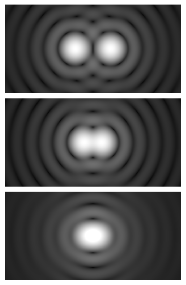
• Rayleigh criterion (isolated features): The lateral distance between two incoherent point sources at which their diffraction patterns are just resolvable is approximately 0.61 · λ / NA.
• Abbe limit (periodic structures): The smallest resolvable period in a line grating for incoherent imaging is approximately λ / (2 · NA). This is equivalent to a cutoff spatial frequency of about 2 · NA / λ in cycles per unit length.
• PSF-based width measures: The full-width at half-maximum (FWHM) of the lateral PSF is often approximated near ~0.5 · λ / NA, which is consistent with the Rayleigh and Abbe perspectives but uses a different width definition.

All of these statements say the same general thing: higher NA and shorter wavelengths enable finer detail. What changes is the numerical constant depending on how you define “just resolved” and whether you consider point-like objects or periodic textures.

Axial resolution and sectioning

Axial resolution (along z) in widefield microscopy scales roughly like n · λ / NA², where n is the refractive index of the imaging medium. The constant in front depends on the exact definition (Rayleigh vs. FWHM) and modality (e.g., widefield vs. confocal). The key takeaway remains: smaller λ, higher NA, and higher index immersion media all shrink the axial PSF, improving sectioning. For 3D imaging, you will link this to z-sampling step size.

Optical transfer function and bandwidth

Every optical microscope can be described by an optical transfer function (OTF), whose magnitude is the modulation transfer function (MTF). The MTF tells you how contrast at each spatial frequency is transmitted. For an ideal, aberration-free, incoherent imaging system, the MTF falls to zero at a cutoff frequency near 2 · NA / λ. Sampling, discussed in Nyquist Sampling, must therefore be fast enough (small pixels in object space) to capture up to this optical bandwidth without aliasing.

Before you worry about pixels and sensors, quantify the optical bandwidth you own. That sets the upper limit for useful sampling density and informs everything that follows.

From Optics to Pixels: Calculating Effective Pixel Size at the Specimen

Digital sampling happens at the camera. But you must think about sampling in specimen space, not in sensor space. The critical quantity is the effective pixel size at the specimen (sometimes called the object-space pixel size). This is the physical size on the sample that corresponds to one camera pixel.

Core formula

The effective pixel size, s_object, is given by

s_object = p_sensor / M_total

where p_sensor is the camera’s pixel pitch (e.g., 6.5 µm) and M_total is the total magnification from specimen to sensor. For typical infinity-corrected systems where the objective magnification is specified for the microscope’s standard tube lens, and where a 1× camera port is used, you can often approximate

M_total ≈ M_objective × M_camera_adapter

with M_camera_adapter the relay optics on the camera port (e.g., 1.0×, 0.63×, 1.5×). If you are using an eyepiece projection or a tube lens different from the nominal design, adjust M_total accordingly using the provided optical factors from the manufacturer. Always confirm how magnifications are defined on your specific stand and adapters.

Interpreting effective pixel size

• Smaller s_object means denser sampling (more pixels per micron), which can capture higher spatial frequencies if the optics provide them.
• Larger s_object means coarser sampling (fewer pixels per micron), which risks aliasing if it undersamples the optical bandwidth.

Once you have s_object, you can compare it to a target object-space sampling interval derived from NA and λ to determine if your setup meets Nyquist sampling.

Worked example (hypothetical numbers)

Suppose your camera has 6.5 µm pixels. With a 40× objective and a 1.0× camera adapter, M_total ≈ 40. Then

s_object = 6.5 µm / 40 = 0.1625 µm per pixel.

Whether this is sufficient depends on the smallest optical detail your 40× objective can resolve at the wavelengths you use. That leads directly to Nyquist.

Nyquist Sampling for Microscopy: How Many Pixels Per Resolution Element?

The Nyquist–Shannon sampling theorem says you need to sample at least twice as fast as the highest spatial frequency you want to capture. In microscopy, the highest spatial frequency your optics deliver is linked to NA and λ (see Numerical Aperture, Wavelength, and Diffraction). Translating that into a practical pixel size yields familiar rules of thumb.

Practical lateral sampling targets

• Using the Rayleigh criterion (0.61 · λ / NA) as the smallest feature of interest, a common target is about 2–3 pixels across that distance. This corresponds to an object-space pixel size of roughly (0.5–0.33) × (0.61 · λ / NA).
• Using the Abbe period (λ / (2 · NA)) for periodic detail, sampling with at least two pixels per period implies an object-space pixel size near λ / (4 · NA). Many practitioners choose slightly finer sampling to accommodate real-world MTF roll-off.

These guidelines are consistent because the different constants pertain to different definitions of “smallest structure.” The central idea is the same: ensure at least two samples per smallest resolvable feature, preferably a bit more to preserve contrast near the cutoff.

Turning a wavelength into a number

To choose a sampling interval, you must decide which wavelength to use. Typical practice is:

• For brightfield (white light), choose a representative wavelength in the green region (e.g., ~550 nm) where many objectives are well corrected and human contrast sensitivity is high.
• For fluorescence, use a representative emission wavelength for the fluorophore signal of interest (e.g., ~520 nm for green emission, ~600–620 nm for orange-red). If multiple channels are imaged, plan around the shortest emission wavelength channel you need to resolve, since it carries higher spatial frequencies.

Example: Does my pixel size meet Nyquist?

Continuing the hypothetical case from effective pixel size with s_object = 0.1625 µm, assume incoherent imaging at λ = 550 nm and NA = 0.75. A Rayleigh-based target spacing might be:

Target spacing ≈ 0.5 × (0.61 · λ / NA) = 0.5 × (0.61 · 0.55 µm / 0.75) ≈ 0.224 µm.

Your sampling at 0.1625 µm/pixel is slightly finer (denser) than this target, which is acceptable and will help preserve contrast near the optical cutoff. If it were much finer (say, 0.05 µm/pixel), you would be oversampling with little gain in resolution but a penalty in SNR and file size. If it were coarser (say, 0.35 µm/pixel), you would undersample and risk aliasing.

Do not forget axial sampling

For 3D stacks, z-step size must also obey Nyquist relative to the axial PSF. A simple rule is to use a z-step of about half the axial resolution measure you adopt. Because axial resolution scales like ~ n · λ / NA², higher NA and shorter wavelengths demand smaller z-steps. Details appear in 3D Imaging and Z-Sampling.

Aliasing, OTF/MTF, and What Goes Wrong When Sampling Is Off

Undersampling does not just “lose detail.” It also creates spurious detail by folding high spatial frequencies into lower ones—a phenomenon called aliasing. In images, aliasing shows up as moiré patterns in periodic textures, false edge orientations, or flickering detail that changes with slight focus or stage motions.

How aliasing happens in microscopy

The microscope forms an analog image in the intermediate image plane and, ultimately, at the camera sensor. The image contains spatial frequencies up to the optical cutoff near 2 · NA / λ (for incoherent imaging under ideal conditions). If the camera sampling frequency in object space is lower than twice that cutoff, frequencies near the cutoff will not be uniquely represented. They fold into lower bands and masquerade as real structure.

Once aliasing is baked into data, there is no reliable post-processing that can reconstruct the true high-frequency content; the information was not sampled adequately. This is why planning your sampling interval is so important.

OTF/MTF and why “perfect Nyquist” still benefits from slight oversampling

The microscope’s MTF drops gradually with frequency; it does not transmit the optical bandwidth uniformly. Contrast near the cutoff is already low. Sampling right at the Nyquist limit risks compressing that fragile high-frequency contrast into just a couple of pixels. A modest oversampling factor (e.g., 10–30% finer than the bare minimum) often preserves edge shapes and enables better downstream processing (e.g., deconvolution) without excessive penalties in SNR and data volume.

Aberrations, coverslips, and real optics

Real objectives are not perfect. Off-specimen coverslip thickness, refractive index mismatch, and misalignment degrade the PSF and reduce effective bandwidth. Ironically, undersampling sometimes looks “fine” when the optics are underperforming, because the real cutoff is lower than theory. That is not a good reason to choose coarse sampling. Instead, tune the optical pathway—cover glass, immersion medium, correction collar, and illumination alignment—so that the optic approaches its design NA and bandwidth. Then set sampling to match.

Oversampling vs. Undersampling: SNR, Speed, and Data Volume Trade-offs

While Nyquist is a mathematical condition, imaging is a practical art that must balance photon budgets, exposure times, readout speeds, and storage. Choosing your sampling rate involves trade-offs.

Costs of oversampling

• Lower SNR per pixel: With a fixed photon flux, smaller object-space pixels collect fewer photons, increasing relative shot noise per pixel.
• Read noise and overhead: More pixels mean more read operations. In low-light regimes, read noise can weigh more heavily.
• Longer frame times or slower readout: For a given camera and region of interest, more pixels often means longer readouts, reducing temporal resolution.
• Data volume: Oversampled datasets consume storage and bandwidth, complicating archiving and analysis.

Costs of undersampling

• Aliasing artifacts and false structure.
• Loss of quantitative fidelity for measurements of feature size, spacing, and morphology.
• Degraded deconvolution performance: Many algorithms assume proper sampling; undersampling starves them of necessary information.

When to consider binning

Hardware binning (on-sensor) or software binning combines adjacent pixels to produce a larger effective pixel. Binning raises SNR per output pixel (more photons summed) at the expense of spatial sampling density.

• In bright conditions where optical resolution limits dominate, binning may throw away useful detail. Avoid unless you are oversampled.
• In dim fluorescence, where read noise and shot noise dominate, modest binning can improve SNR and speed without harming resolution—if you remain at or above Nyquist relative to the optical cutoff. Evaluate this with your effective pixel size and target sampling interval.

Trade-offs differ by modality

• Brightfield/phase contrast/DIC: Often bright enough to run near the ideal Nyquist sampling for the objective’s NA.
• Fluorescence: Photon-limited. Slight undersampling may be acceptable for screening and speed, but quantitative work should respect Nyquist to the extent practical.
• Confocal and other scanning systems: Sampling is set by scan step sizes, discussed in 3D Imaging and Z-Sampling; the same Nyquist logic applies.

Field of View, Sensor Size, and Camera Couplers: Matching Optics to Silicon

Beyond sampling density, you must also ensure that the field of view (FOV) projected onto the sensor is appropriate for your specimen and that the optical image circle is used efficiently.

Image circle and camera sensor

Most modern objectives are designed to produce a flat, corrected image over a specified field number at the intermediate image plane. The camera adapter optics project part of that field onto the sensor. Using a camera with a sensor larger than the corrected field may result in vignetting or degraded off-axis performance, while using a very small sensor may waste the available field and force higher magnification than needed, impacting SNR and speed.

Choosing a camera adapter magnification

Camera port adapters (e.g., 0.5×, 0.63×, 1×, 1.5×) trade field of view against sampling density:

• Lower adapter magnification (e.g., 0.5×) projects a larger field onto the sensor, increasing FOV but coarsening object-space pixel size (larger s_object), which can push you below Nyquist. Verify with effective pixel size calculations.
• Higher adapter magnification (e.g., 1.5×) reduces FOV but refines object-space pixel size (smaller s_object), which can help reach Nyquist on cameras with large pixels but may oversample and cost SNR.

Practical considerations for matching optics and sensor

• Start with the objective NA and wavelength to compute a target sampling interval.
• Use camera pixel size and adapter magnification to compute s_object.
• Adjust the adapter if needed to land near your Nyquist target while keeping an adequate FOV for your specimen.
• Confirm that the resulting FOV lies within the corrected image circle of your objective and camera path.

Color Cameras, Bayer Patterns, and Resolution Penalties

Color cameras achieve color by placing a mosaic of color filters (often a Bayer pattern of red, green, and blue) over the sensor. Each pixel records only one color channel, and the missing channels are reconstructed by demosaicing. This affects sampling and resolution in several ways.

Bayer sampling is not uniform across colors

• The green channel is sampled more densely (typically half of the pixels in a Bayer RGGB pattern), while red and blue are sampled more sparsely (quarter each). Effective resolution can therefore differ by color channel.
• Demosaicing algorithms interpolate missing color samples, which smooths fine detail and can suppress high-frequency contrast compared with a monochrome sensor of the same pixel pitch.

Implications for sampling choices

• If your application values maximum spatial resolution and quantitative fidelity, a monochrome camera with appropriate filters generally preserves higher contrast at fine spatial frequencies than a comparable color camera.
• When using color cameras for brightfield, you may need to sample slightly finer in object space to offset demosaicing losses, especially if resolving fine periodic textures prone to moiré.
• For fluorescence, color cameras are typically less suitable because the emission bands are recorded through color filters not optimized for narrowband emission. Monochrome sensors with emission filters are standard for quantitative fluorescent imaging.

3D Imaging and Z-Sampling: Axial Resolution and Step Size

In 3D datasets (widefield stacks, confocal scans), you must also sample along z. The axial PSF is elongated relative to the lateral PSF, so axial sampling intervals are usually larger than lateral ones for the same objective.

Axial resolution scaling

For widefield imaging, axial resolution scales approximately like ~ n · λ / NA². The exact constant depends on the criterion (Rayleigh vs. FWHM) and imaging modality. For confocal with a small pinhole, axial resolution is typically improved relative to widefield and follows a similar inverse-square dependence on NA.

Choosing a z-step

• A practical rule is to set the z-step to about half of your chosen axial resolution measure. This is the axial analogue of Nyquist sampling.
• If you intend to use deconvolution on widefield stacks, sampling slightly finer than this rule can help algorithms recover axial detail more reliably, provided SNR is sufficient.
• For confocal and other point-scanning systems, ensure the lateral scan step and the z-step both meet Nyquist for the system’s effective PSF. Manufacturers often provide recommended step sizes based on NA and wavelength; verify these against the Nyquist logic presented here.

Refractive index mismatches

Imaging deep into specimens with refractive index heterogeneity distorts the axial PSF and can introduce spherical aberration, effectively worsening axial resolution and changing the optimal z-step. To the extent possible, match immersion media and mounting media to minimize aberrations. When in doubt, evaluate measured PSFs (e.g., fluorescent beads) to ground your z-step decision in experimental data.

Practical Workflows: Objective–Camera–Adapter Combinations That Make Sense

Connecting the formulas to real decisions is where most users need guidance. Below are stepwise workflows to choose lateral and axial sampling that respect optical limits while keeping data practical.

Workflow A: Brightfield with a mid-NA objective

1. Define the optical target: Suppose you use a 40×/0.75 NA objective for brightfield at a representative λ = 550 nm.
2. Compute a lateral sampling goal: Rayleigh-based minimum spacing 0.61·λ/NA ≈ 0.61·0.55 / 0.75 ≈ 0.447 µm. Target object-space pixel size near 0.5 × that ≈ 0.22 µm/pixel (2 pixels across Rayleigh distance) or slightly finer.
3. Pick a camera and adapter: With 6.5 µm pixels and 1.0× adapter, s_object ≈ 6.5/40 ≈ 0.1625 µm/pixel. That is a modest oversample compared with the 0.22 µm target—good for preserving high-frequency contrast.
4. Check FOV: Ensure the resulting field matches your specimen needs. If you need more field, a 0.75× adapter would give s_object ≈ 0.216 µm/pixel—right on target—but increases FOV. Make sure vignetting is not introduced.

Workflow B: Green fluorescence with a high-NA oil objective

1. Objective: 60× oil, NA = 1.4. Emission near 520 nm.
2. Lateral target: Rayleigh spacing 0.61·0.52 / 1.4 ≈ 0.226 µm. Two pixels per Rayleigh distance gives ~0.113 µm/pixel. Many users choose ~0.09–0.11 µm/pixel to modestly oversample.
3. Camera match: With a 6.5 µm pixel and 1.0× adapter, s_object ≈ 6.5/60 ≈ 0.108 µm/pixel—a good match. If your camera pixels are larger (e.g., 11 µm), consider a higher adapter magnification (e.g., 1.5×) to achieve ~0.122 µm/pixel (11 / (60 × 1.5)).
4. Axial sampling: Estimate axial resolution scaling with ~ n·λ/NA² (n ≈ 1.515 for oil). Choose a z-step near half that value to satisfy axial Nyquist (see z-sampling), adjusting for SNR and deconvolution plans.

Workflow C: Survey imaging where speed matters

1. Define acceptable loss: If your goal is to scan large areas quickly to find regions of interest, modest undersampling might be acceptable, provided you understand the risk of aliasing with fine textures.
2. Tune adapter: Use a lower adapter magnification (e.g., 0.5× or 0.63×) to increase FOV per frame, while checking s_object stays near or just above the Nyquist target for your objective/λ. If it falls well below Nyquist, plan to re-image the ROI at proper sampling later.
3. Exploit binning: If SNR is limiting, bin to increase frame rate and SNR. Confirm that your binned s_object still meets the reduced sampling requirements of your survey task.

Workflow D: Color brightfield with a Bayer sensor

1. Expect reduced fine-detail contrast compared with monochrome at the same pixel pitch due to demosaicing.
2. Sample slightly finer than the bare minimum to offset the resolution penalty, especially if diagnosing periodic aliasing patterns (e.g., in textiles, printed materials, or organized biological tissues).
3. Validate visually: Slight adjustments in adapter magnification may be needed to balance FOV and sampling while maintaining robust color fidelity.

Workflow E: Quantitative measurements and scale bars

1. Calibrate pixel size at the specimen using a stage micrometer or certified calibration slide. Do not rely solely on nominal magnifications.
2. Verify linearity across the field if you plan to measure areas or lengths off-axis.
3. Report sampling in your notes or figure captions (e.g., “0.108 µm/pixel; z-step 0.3 µm”). This transparency aids reproducibility.

Frequently Asked Questions

Is it ever acceptable to undersample on purpose?

Yes—if your goal is rapid screening or qualitative observation and your specimen lacks fine periodic detail susceptible to aliasing. In such cases you can trade spatial fidelity for speed and lower data volume. However, for quantitative work or when fine textures matter, you should adhere to Nyquist sampling. If you undersample at acquisition, post-processing cannot fully restore lost or aliased information.

How does digital zoom differ from optical magnification for sampling?

Digital zoom simply interpolates or enlarges existing pixels; it does not change object-space sampling density. Optical magnification (objective and adapter) changes the mapping between specimen space and sensor pixels and therefore directly alters effective pixel size. If you need more sampling density, adjust optical magnification or choose a camera with smaller pixel pitch—not digital zoom.

Glossary of Key Terms for Digital Microscopy Sampling

• Numerical aperture (NA): A dimensionless measure of an objective’s light-gathering ability and angular acceptance. Higher NA improves resolution and brightness for a given wavelength.
• Wavelength (λ): The distance between successive peaks of a light wave. Shorter wavelengths carry higher spatial frequencies and resolve finer detail, all else equal.
• Point spread function (PSF): The intensity distribution produced by a point source in the image. Its width defines resolution limits and informs Nyquist sampling.
• Optical transfer function (OTF): The Fourier transform of the PSF; it describes how spatial frequencies are transmitted. Its magnitude is the modulation transfer function (MTF).
• Rayleigh criterion: A lateral resolution criterion for incoherent imaging stating that two point sources are just resolved when the principal maximum of one diffraction pattern coincides with the first minimum of the other, approximated by 0.61 · λ / NA.
• Abbe limit: A resolution limit for periodic structures in incoherent imaging, with smallest resolvable period approximately λ / (2 · NA).
• Nyquist sampling: The minimum sampling rate needed to capture a signal without aliasing; at least twice the highest frequency present.
• Aliasing: The misrepresentation of high spatial frequencies as lower ones due to insufficient sampling.
• Effective pixel size at the specimen: The real-world size on the sample that corresponds to a single camera pixel, computed as p_sensor / M_total.
• Binning: Combining adjacent pixels to form a larger effective pixel, improving SNR per pixel but reducing sampling density.

Final Thoughts on Choosing the Right Sampling Strategy for Digital Microscopy

Sampling and resolution in digital microscopy come down to a simple, rigorous chain: the objective’s NA and the wavelength set an optical bandwidth; the camera pixel pitch and adapter magnification translate that bandwidth into a required object-space pixel size; and the Nyquist criterion defines the minimum sampling interval to capture it faithfully. Around that chain, real-world considerations—SNR, field of view, color filter arrays, 3D z-steps, and data volume—shape practical choices.

Use the following concise checklist as you plan an imaging setup or session:

• Determine a representative λ for your modality and channel(s).
• Compute a lateral resolution measure (e.g., 0.61·λ/NA) and pick a target sampling interval of roughly half that value.
• Calculate effective pixel size from your camera and adapter. Adjust the adapter if needed to land near your target.
• Set z-step size to about half your chosen axial resolution measure for 3D stacks.
• Account for color camera penalties, binning and SNR trade-offs, and the field of view you need.
• Verify with a calibration slide or bead sample, and document your sampling for reproducibility.

With these principles, you can align optics and detector to the physics of diffraction and the mathematics of sampling—capturing images that are not just sharp, but also faithful to the specimen and robust for measurement. If you found this deep dive useful, consider exploring our related articles on optical aberrations, contrast mechanisms, and image processing fundamentals. Subscribe to our newsletter to receive future installments on microscope fundamentals, types, accessories, and applications.