
Table of Contents
- What Are Infinity-Corrected and Finite-Conjugate Microscope Systems?
- Optical Paths and Image Formation in Finite and Infinity Designs
- Magnification, Numerical Aperture, and Resolution in Each System
- Aberrations, Field Flatness, and Optical Corrections
- Accessories, Infinity Space, and Modular Optics
- Component Compatibility and Mixing Finite and Infinity Parts
- Use Cases, Trade-Offs, and Choosing Between Systems
- Practical Calculations and Worked Examples
- Setup, Alignment, and Imaging Considerations
- Frequently Asked Questions
- Final Thoughts on Choosing the Right Microscope Optical System
What Are Infinity-Corrected and Finite-Conjugate Microscope Systems?
Optical microscopes broadly follow two architectures for how objectives create images: finite-conjugate and infinity-corrected. Both systems aim to form a sharp, high-contrast intermediate image that can be viewed through eyepieces or projected to a camera. The difference lies in how the objective lens delivers that intermediate image and how the rest of the optical train completes the imaging task.
In a finite-conjugate system, the objective directly forms a real intermediate image at a specific, finite distance behind it. Historically, manufacturers defined a mechanical tube length—commonly on the order of 160 mm or 170 mm—for which the objective’s aberrations were corrected and its magnification specification was valid. This finite distance ends at the plane where the eyepiece or camera relay picks up the image for further magnification or detection.
Artist: Rama
In an infinity-corrected system, the objective emits nearly collimated (parallel) light for an object in focus. A separate tube lens then focuses this collimated beam to form the intermediate image inside the microscope body. The nominal objective magnification is defined with respect to a particular tube lens focal length. By placing optical components in the parallel “infinity space” between the objective and the tube lens, one can insert beam-splitting prisms, contrast modules, or filters with minimal impact on focus.
From a user’s perspective, both systems can deliver superb images. The distinctions show up in modularity, compatibility with accessories, and how magnification is defined and maintained. If you are choosing a stand or planning to mix components, understanding these differences is essential. If you want more on how magnification and NA relate across designs, see Magnification, Numerical Aperture, and Resolution in Each System.
Optical Paths and Image Formation in Finite and Infinity Designs
To understand how these systems differ, it helps to think about conjugate planes—pairs of object and image planes where a sharp image forms. Microscopes typically have two principal conjugates: the specimen plane and the intermediate image plane. Eyepieces and cameras view this intermediate image, not the specimen directly.
Finite-conjugate pathway
In a finite system, the objective is designed to create a real intermediate image at a fixed distance behind the objective shoulder. The mechanical tube length defines where that image should fall for optimal correction. Eyepieces in many finite systems historically played a role in correcting residual lateral chromatic aberration and field curvature, which is why “compensating” eyepieces were often paired with certain finite objectives.
Object -----> [Objective] === finite distance ===> [Intermediate Image] -> [Eyepiece/Camera]

Artist: Gilles San Martin
A practical implication: altering the tube length or inserting optics between the objective and the intermediate image plane changes the distance and the aberration balance the objective expects. That can degrade image quality and alter magnification in ways not intended by the design.
Infinity-corrected pathway
In an infinity-corrected microscope, the objective forms an image “at infinity,” which means outgoing rays from a point in the specimen are rendered nearly parallel. A tube lens—effectively a relay lens set at a particular focal length—then brings these parallel rays to focus at the intermediate image plane.
Object -----> [Objective] =>=>=> (parallel/infinity space) =>=>=> [Tube Lens] -> [Intermediate Image] -> [Eyepiece/Camera]

Artist: QuodScripsiScripsi
This architecture creates a region of parallel light commonly called the infinity space. Non-focusing components—like beam splitters, polarizers, fluorescence filter cubes, or differential interference contrast (DIC) prisms—can be inserted in this space without shifting the focus. That modularity is a key advantage for research stands and custom imaging rigs. For a deeper look at accessories and their placement, jump to Accessories, Infinity Space, and Modular Optics.
Intermediate image and viewing
In both systems, the intermediate image is eventually re-imaged by the eyepiece for visual observation or coupled into a camera via a projection lens. This means that many aspects of visual ergonomics (eyepiece magnification, field number, focusability) and camera coupling (sensor size, relay magnification) are similar in spirit, even if the internal routes differ. However, how magnification is defined and maintained differs between the two, as we explain in Magnification, Numerical Aperture, and Resolution in Each System.
Magnification, Numerical Aperture, and Resolution in Each System
Microscope performance is governed by three interrelated concepts: magnification, numerical aperture (NA), and resolution. Understanding how they connect will help you evaluate objectives regardless of whether your stand is finite or infinity-corrected.
Objective magnification and system magnification
- Finite-conjugate systems: The objective’s marked magnification assumes a specified mechanical tube length and a matched eyepiece design. Changing the tube length or using an eyepiece with different characteristics can alter the effective magnification and aberration balance.
- Infinity-corrected systems: The objective magnification is defined relative to a particular tube lens focal length. The basic relationship is Mobjective ≈ ftube / fobjective. If a 10× objective is specified using a certain tube lens focal length, changing that focal length scales the effective magnification proportionally. Manufacturers publish the tube lens focal length for which their objective magnifications are specified.
For visual observation, total magnification is approximately the product of the objective magnification and the eyepiece magnification (e.g., 40× objective with 10× eyepiece yields 400×). For cameras, one often describes the on-sensor magnification, which depends on the camera relay optics (if any) and the sensor size relative to the intermediate image size.
Numerical aperture (NA) and resolution
NA measures the objective’s acceptance cone of light and directly ties to lateral resolution and light-gathering power. Under incoherent brightfield conditions, the diffraction-limited lateral resolution can be estimated by d ≈ 0.61 λ / NA, where λ is the imaging wavelength. Higher NA means finer detail can be resolved and brighter images (all else equal) due to greater light collection.
Artist: Ice Boy Tell
- Key point: Whether your microscope is finite or infinity-corrected does not, by itself, change the diffraction limit. Resolution is primarily set by NA and wavelength, plus the quality of correction across the field.
- Illumination coherence: Changing illumination conditions (e.g., phase contrast, darkfield, or highly coherent illumination) modifies the effective resolution and contrast transfer, but this is independent of the finite vs infinity distinction.
Field of view and field number
Eyepieces have a field number (FN) that indicates the diameter of the field stop in millimeters at the intermediate image plane. The specimen-plane field diameter is approximately FN divided by the objective magnification. In practical systems, relay optics, camera ports, and field-flattening elements also influence how much of that field is delivered uniformly to your eye or sensor.
In finite microscopes, the objective directly determines the intermediate image scale at the specified tube length. In infinity systems, the tube lens focal length governs that scale. Either way, you can estimate the field of view on the specimen by combining the objective magnification with the eyepiece FN and any relay magnification in the camera path. For worked examples of these relationships, see Practical Calculations and Worked Examples.
Aberrations, Field Flatness, and Optical Corrections
Real lenses have aberrations—chromatic, spherical, coma, astigmatism, field curvature, and distortion—that must be balanced to deliver a flat, sharp, high-contrast image. Objectives, eyepieces, and tube lenses share these correction burdens differently depending on the microscope architecture and the era of design.
Objective classes and correction goals
- Achromats: Correct for two wavelengths (typically in the visible range) for axial chromatic aberration and provide modest field flatness. Widely used for routine brightfield.
- Plan achromats: Achromat color correction with improved field flatness—the image stays in focus across a larger diameter of the field.
- Fluorites (semi-apochromats): Better chromatic and spherical correction than achromats, often with higher NA for fluorescence and contrast methods.
- Apochromats: Correct axial chromatic aberration for three or more wavelengths with tight control of spherical aberration; typically provide the highest NA and best color correction at a premium.
These labels describe correction performance and exist in both finite and infinity objectives. The finite vs infinity difference is mainly about where the intermediate image is formed and how other optics contribute to corrections.
Correction sharing: finite vs infinity
- Finite-conjugate tradition: Many finite systems historically relied on compensating eyepieces to neutralize residual lateral chromatic aberration and field curvature left by the objective. Swapping eyepieces designed for one objective family into another system could expose color fringes or field curvature because the intended correction pair was broken.
- Infinity-corrected designs: Modern infinity systems tend to push more correction into the objective and tube lens pair, allowing relatively neutral eyepieces that primarily magnify without adding significant aberration shaping. That said, details vary: some systems distribute corrections between objective and tube lens in proprietary ways.
The practical consequence is compatibility. Mixing a finite objective that expects a compensating eyepiece into a system with a neutral eyepiece can produce lateral color and off-axis blur. Conversely, using an infinity objective with an unsuitable tube lens focal length can alter magnification and induce field-dependent aberrations. For a dedicated discussion of mixing components, head to Component Compatibility and Mixing Finite and Infinity Parts.
Field flatness and planarity
Field flatness—the ability to keep the image in focus across the entire field—is addressed by both objective design and auxiliary optics. Plan objectives (e.g., plan achromat, plan apochromat) are optimized for a flatter, more uniform field. Whether your microscope is finite or infinity does not guarantee planarity; you must select the objective grade that matches your field uniformity needs.
Coverslip correction and working distance
- Coverslip thickness: Many biological objectives are designed for a nominal coverslip thickness around 0.17 mm (often marked on the barrel). Deviations can introduce spherical aberration, reducing contrast and resolution. This is independent of finite vs infinity.

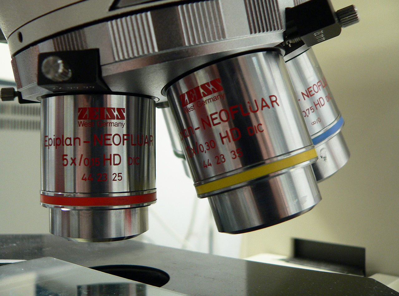
Microscope objective marking (Zeiss oil immersion objective CP-Achromat 100x/1.25): \”CP-Achromat\” describes the type of objective with regard to the correction of optical aberrations. An achromat is an optical system consisting of at least two lenses that reduces chromatic aberration (color errors for light of different wavelengths). The \”C\” is used for achromatic lenses that produce good image contrast. The \”P\” stands for \”plan\” (flat) and indicates that the optical field curvature that occurs with simple lenses has been corrected, so that flat specimens are imaged sharply in the center and at the edges simultaneously. \”100x\” indicates that the optical magnification factor of the intermediate image is 100 (with a suitable tube lens). \”1,25 Oil\” (with a German decimal separator = comma) indicates the numerical aperture 1.25 (a measure of spatial resolution) achieved with immersion oil. Only with oil immersion, the objective provides a good image. The infinity symbol shows that the objective lens was designed for microscopes with an infinity beam path. \”0,17\” indicates that coverslips with a thickness of 0.17 mm must be used.
Artist: QuodScripsiScripsi - Working distance (WD): The clearance between the front lens and the specimen is set by objective design (e.g., long-working-distance variants), not by whether the system is finite or infinity-corrected.
Accessories, Infinity Space, and Modular Optics
One of the most visible differences between finite and infinity systems is how accessories fit into the optical path. In an infinity-corrected microscope, the collimated region between the objective and tube lens allows you to insert devices without introducing unintended focusing power.
Common accessories that benefit from infinity space
- Beam splitters and trinocular heads: Divert some light to a camera without changing the focal position at the intermediate image.
- Contrast modules: Polarizers, analyzers, and DIC prisms can be placed in the infinity space where they modify polarization or phase without adding focus shift.
- Fluorescence filter cubes: Excitation filters, dichroic mirrors, and emission filters are stacked in turrets situated inside the infinity space to enable rapid channel switching.
- Insertion of additional optics: Optional magnifiers, telecentric relays, or beam conditioning optics can sometimes be placed here, provided their design maintains collimation or is accounted for in the system layout.
In finite systems, placing refractive elements between the objective and the intended intermediate image plane typically changes the optical path length, potentially upsetting aberration corrections and focus. Some accessories in finite microscopes are therefore placed in conjugate planes that minimize disruption, or they are designed to compensate for their own optical power.
Telecentricity considerations
In imaging and metrology, telecentricity (rays entering the lens being parallel to the optical axis in image or object space) can reduce perspective errors and magnification changes with focus. Infinity-corrected architectures make it straightforward to design telecentric relays in the infinity space, but standard microscope objectives are not necessarily telecentric by default. Specialized objectives and relays are used when strict telecentric imaging is required.
For users building custom optical trains—say, inserting a laser combiner for fluorescence or adding a beam splitter for simultaneous dual cameras—the collimated segment in infinity designs simplifies integration. If you plan to do this, coordinate with the system’s tube lens focal length and back focal requirements described in Magnification, Numerical Aperture, and Resolution in Each System and confirm compatibility notes in Component Compatibility and Mixing Finite and Infinity Parts.
Component Compatibility and Mixing Finite and Infinity Parts
Microscope optics are precision-matched. While adapters exist, mixing parts across systems (and across manufacturers) is rarely plug-and-play. Here are the core compatibility points to understand before attempting a hybrid system.
Parfocal distance, threading, and mechanical fit
- Thread standard: Many objectives use a common threading (for example, a 20.32 mm diameter with 36 TPI is widespread), but not universal. Always verify the actual thread and mechanical interface.
- Parfocal distance: Objectives are designed to come into focus at a standard distance from the nosepiece face. Common parfocal distances include around 45 mm and around 60 mm, among others. Mixing objectives with different parfocal distances may require refocusing when switching magnifications and can limit compatibility with nosepieces and condensers.
Optical compatibility warnings
- Finite objective on an infinity stand: Without the correct optical path length, a finite objective will not deliver its intended magnification or correction. Placing a finite objective ahead of a tube lens can make it behave like a short-focal-length lens rather than an objective corrected for a fixed tube length, often yielding significant aberrations.
- Infinity objective without the right tube lens: The effective magnification becomes ftube/fobjective. Using a tube lens with a focal length other than the specified standard changes magnification and can alter off-axis performance. Certain correction terms may be distributed between the objective and a matched tube lens.
- Compensating vs neutral eyepieces: If an eyepiece was designed to correct residual aberrations (common in many finite-era systems) and you pair it with fully corrected optics, you may overcorrect and introduce color fringes. Conversely, using a neutral eyepiece with an objective that expected compensating corrections can leave lateral color uncorrected.
Camera couplers and projection optics
Camera adapters typically provide a relay lens that projects the intermediate image onto a sensor of known size. In both finite and infinity microscopes, the camera path must be designed to match the intermediate image size and keep aberrations well-controlled across the sensor. If you see edge softness or color fringes only on the camera, the camera relay may be the culprit rather than the objective.
In trinocular infinity systems, a beam splitter commonly diverts a fraction of the infinity beam to the camera port before the tube lens. A dedicated camera tube lens or relay then completes the imaging onto the sensor. In finite systems, the camera is frequently coupled closer to the eyepiece or intermediate image plane, and specific projection factors are used to achieve the desired on-sensor magnification. For numeric illustrations, see Practical Calculations and Worked Examples.
Use Cases, Trade-Offs, and Choosing Between Systems
Both finite and infinity-corrected microscopes can be the right choice depending on your goals, budget, and need for modularity. Below are common decision criteria for educators, hobbyists, and research users.
When finite-conjugate systems make sense
- Teaching and basic inspection: For straightforward brightfield work, finite microscopes offer excellent value. The lack of a tube lens means fewer optical components in the body and often a lower cost for a complete setup.
- Fixed configurations: If you rarely add or change contrast modules, the finite design’s simplicity can be an advantage. Less complexity can mean fewer alignment steps and fewer variables to drift.
- Legacy ecosystems: If you already own compatible finite objectives and compensating eyepieces and you are satisfied with the image quality, continuing with finite may be more economical, especially for routine tasks.
When infinity-corrected systems shine
- Modularity and accessories: If you plan to use DIC, epi-fluorescence, beam splitters, or custom optical modules, the infinity space supports insertion without altering focus. This modularity is central to many research-grade stands.
- Camera integration: Trinocular heads and camera ports are widely supported with well-matched relay optics in infinity systems, simplifying documentation and digital imaging.
- Objective families and upgrades: Many modern objectives—especially high-NA apochromats and specialized long-working-distance types—are designed for infinity systems. Upgrading across a current objective line may be easier when tube lens standards are stable.
Trade-offs to weigh carefully
- Cost and complexity: Infinity systems typically cost more and include more optical elements. The upside is modularity; the downside is budget and the need to ensure all parts match the tube lens standard.
- Compatibility risk: Mixing components across generations or manufacturers is risky. A carefully matched finite system can outperform a mismatched infinity setup if the latter’s components are not optically compatible.
- Serviceability: Simpler finite stands may be easier to maintain. Complex infinity stands with multiple modules demand more careful alignment and dust control in the infinity space.
If you are torn between the two, list the accessories and imaging modes you plan to use in the next several years. If the list includes modular fluorescence, advanced contrast, or multi-camera paths, the flexibility described in Accessories, Infinity Space, and Modular Optics often tips the scales toward infinity-corrected stands.
Practical Calculations and Worked Examples
Let’s make the relationships concrete with practical calculations. These examples are illustrative and rely on standard relationships commonly used in optical microscopy. Always confirm the exact specifications from your microscope or objective documentation.
Example 1: Infinity objective magnification with different tube lenses
Suppose an infinity-corrected objective is marked 10× at a specified tube lens focal length of 200 mm. The objective’s effective focal length is then fobjective ≈ 200 mm / 10 = 20 mm (conceptually). If you used a 180 mm tube lens instead, the effective magnification becomes M ≈ 180 mm / 20 mm = 9×. Two consequences follow:
- The specimen looks slightly less magnified (9× versus 10×).
- The field of view increases proportionally, assuming the eyepiece field stop and camera relay can deliver the wider field without vignetting.
However, it is not just magnification that changes. Off-axis corrections are usually optimized for the specified tube lens focal length. Deviating from it can subtly affect edge performance. That is why mixing objectives with tube lenses from different ecosystems is not guaranteed to preserve planarity or color correction.
Example 2: Field of view from eyepiece field number
Let’s say an eyepiece has a field number FN = 20 mm. With a 40× objective, the approximate specimen-plane field diameter is FN / M ≈ 20 mm / 40 = 0.5 mm. If you switch to a 20× objective, the field diameter doubles to ~1.0 mm (again, approximations; actual delivered field depends on the relay optics and whether the objective maintains quality across that larger field).
This rule-of-thumb holds similarly in finite and infinity systems, but make sure your system actually illuminates and relays that field without vignetting. Illumination and relay optics need to be sized accordingly; see Setup, Alignment, and Imaging Considerations.
Example 3: Camera on-sensor magnification
Imagine you have a camera with a 6.4 mm-wide sensor. Through a 10× objective and a camera relay that produces 1× at the sensor, the on-sensor field width corresponds to the intermediate image width divided by relay magnification. If the eyepiece or camera relay is designed to project the full FN = 18 mm field to the camera without cropping, then the sensor will capture only a fraction of that diameter. The specimen width on the sensor is approximately (sensor width / objective magnification) if the relay is 1×. So 6.4 mm / 10 ≈ 0.64 mm span on the specimen. If you change the relay to 0.5×, you double the captured specimen width to ~1.28 mm.
These estimates assume the relay is properly matched to the intermediate image size and that the system supports the desired field without aberration growth at the edges.
Example 4: Resolution and NA
Suppose you use green light at λ ≈ 550 nm with a 0.65 NA objective. The diffraction-limited lateral resolution is approximately d ≈ 0.61 × 0.55 µm / 0.65 ≈ 0.52 µm. If you switch to a 0.95 NA objective, d improves to ≈ 0.35 µm. These numbers do not depend on whether your system is finite or infinity-corrected; they depend on NA and wavelength. Image quality also depends on aberration control across the field and precise alignment, discussed further in Aberrations, Field Flatness, and Optical Corrections and Setup, Alignment, and Imaging Considerations.
Example 5: Effect of coverslip mismatch
If an objective is corrected for a 0.17 mm coverslip but you use a significantly different thickness, spherical aberration can reduce contrast and resolution. This is architecture-agnostic: finite and infinity objectives alike rely on the correct optical path near the specimen. When in doubt, use coverslips matching the objective’s marking or select objectives with adjustable correction collars designed for varying coverslip thicknesses.
Setup, Alignment, and Imaging Considerations
Whether your microscope is finite or infinity-corrected, careful setup and alignment pay dividends in image quality. The fundamentals remain consistent because both architectures create an intermediate image that eyepieces or cameras view.
Illumination alignment
- Köhler illumination: A properly adjusted condenser and field iris provide even, glare-free illumination and optimal contrast. This applies equally to both finite and infinity stands.
- Condenser matching: Match the condenser NA to the objective NA for bright, high-resolution images. Underfilling the objective pupil can increase contrast at the expense of resolution; overfilling can add stray light.
Parfocality and objective switching
Using objectives with a common parfocal distance keeps specimens in focus when changing magnification. If you mix objectives with different parfocal distances, expect to refocus. In some cases, spacers or adjustable nosepieces can mitigate differences, but best results come from matched objective sets.
Camera coupling and sampling
For digital imaging, sensor sampling should be adequate for the optical resolution. A rule of thumb is to sample at least twice (often closer to 2–3×) the spatial frequency associated with the optical resolution limit. Practically, this means selecting camera pixel sizes and relay magnifications that produce a pixel size at the specimen on the order of d/2 to d/3, where d is the diffraction-limited resolution. This ensures you capture the resolvable detail without undersampling.

Artist: Martin Cooper from Ipswich, UK
Cleanliness and dust control
Dust and smudges anywhere in the beam path reduce contrast. In infinity systems, dust in the infinity space may project softly into the image depending on placement; in finite systems, dust near conjugate image planes can appear more sharply. Keep objectives, tube lenses, and eyepieces clean with appropriate, non-abrasive methods.
Mechanical stability
Vibration and drift affect all microscopes. Infinity systems with many modules can be slightly more sensitive to internal alignment, while finite systems can be more compact. In either case, a rigid stand, stable table, and minimal air currents help preserve resolution and repeatability—especially at higher magnifications.
Frequently Asked Questions
Can I use a finite objective on an infinity-corrected microscope (or vice versa)?
Not directly, and not without trade-offs. A finite objective expects a specific mechanical tube length and often a compensating eyepiece to complete its aberration correction. Putting it in front of a tube lens (in an infinity stand) generally leads to incorrect magnification and aberrations. Conversely, an infinity objective requires the correct tube lens focal length to produce its specified magnification and aberration performance. There are adapters and specialized relays for certain cross-uses, but success depends on careful optical design and may not match the performance of a native, matched system. For more, see Component Compatibility and Mixing Finite and Infinity Parts.
Does choosing infinity-corrected optics automatically improve resolution?
No. Resolution primarily depends on numerical aperture and wavelength, along with the quality of aberration correction across the field. Infinity-corrected systems provide modularity and flexibility but do not inherently change the diffraction limit. A well-corrected finite objective with appropriate illumination and coverslip control can rival an infinity objective of comparable NA and grade. To review how NA and magnification relate to resolution, visit Magnification, Numerical Aperture, and Resolution in Each System.
Final Thoughts on Choosing the Right Microscope Optical System
The choice between infinity-corrected and finite-conjugate microscopes comes down to how you plan to use your instrument. Infinity-corrected designs excel when you need modular accessories, flexible camera integration, and a broad upgrade path. Finite systems offer compelling simplicity and value for routine brightfield and teaching labs where configurations remain stable. In both cases, ultimate image quality is governed by objective NA and correction grade, proper illumination, and precise alignment.
If your roadmap includes advanced contrast techniques, fluorescence, multi-camera outputs, or custom optical modules, the parallel beam region in an infinity system can simplify your build and preserve focus when inserting accessories. If you prioritize cost, ease of use, and a compact footprint for straightforward imaging, a well-matched finite setup is hard to beat.
Whichever route you choose, match objectives, eyepieces, and (for infinity systems) the tube lens as a coherent set. Pay attention to parfocal distance, field number, and camera coupling to avoid vignetting and edge aberrations. With these fundamentals, you will capture the full performance your optics can deliver.
Looking for more deep dives into microscopy principles? Explore our related topics on optical contrast methods, numerical aperture, and field-of-view optimization—and subscribe to our newsletter to get future articles like this one delivered to your inbox.