Table of Contents
- What Is Numerical Aperture (NA) and Why It Matters
- Optical Resolution Limits: Abbe and Rayleigh Criteria
- Magnification Myths, Empty Magnification, and Useful Range
- Illumination, Coherence, and Condenser NA Matching
- Camera Pixel Size, Sampling, and Nyquist in Microscopy
- Depth of Field and Axial Resolution: How NA Controls Z
- Immersion Media: Air, Water, and Oil Objectives
- Common Misconceptions and How to Check Your Optics
- Frequently Asked Questions
- Final Thoughts on Choosing the Right NA and Magnification
What Is Numerical Aperture (NA) and Why It Matters
In light microscopy, numerical aperture (NA) is the single most important specification for understanding how much detail your system can resolve. While magnification shows you a larger image, NA determines how much information makes it into that image. In practice, higher NA means finer spatial detail (higher resolution), brighter images at the same exposure, and shallower depth of field. NA links the geometry of light collection to the fundamental diffraction limit imposed by wave optics.
Formally, numerical aperture is defined as:
NA = n · sin(θ)
Artist: Happie1Soul
where:
- n is the refractive index of the medium between specimen and objective front lens (≈1.00 for air, ≈1.33 for water, ≈1.515 for many immersion oils).
- θ is the half-angle of the largest cone of rays that can enter (or exit) the objective.
Because sin(θ) ≤ 1, the maximum achievable NA in air is limited to about 1.0 (practically a bit lower). Using higher-index immersion media allows NA greater than 1.0. For example, oil-immersion objectives commonly advertise NA ≈ 1.25–1.45. The key takeaway: all else equal, a larger NA gathers light from higher angles, capturing higher spatial frequency content of the specimen’s diffraction pattern and therefore supporting finer resolution. This section sets the stage; the mathematical connection between NA and resolution is elaborated in Optical Resolution Limits: Abbe and Rayleigh Criteria.
NA is a property of both the objective and, for transmitted-light modalities like brightfield, the condenser. The objective’s NA governs the imaging system’s acceptance of fine details; the condenser’s NA governs the illumination cone that excites or transmits through the sample. In brightfield, matching condenser NA to objective NA is important for achieving the maximum theoretical resolution and contrast (more on this in Illumination, Coherence, and Condenser NA Matching).
Beyond resolution, NA influences several practical aspects of image quality:
- Image brightness: For a given magnification and exposure, higher NA generally yields a brighter image due to a larger photon collection solid angle.
- Depth of field (DOF): Higher NA reduces DOF, giving a thinner optical section in focus. This is beneficial for resolving fine lateral detail but demands careful focusing.
- Working distance: High-NA objectives often have smaller working distances (distance from the front lens to the specimen), reflecting the need for a large collection angle and strong lens curvature.
- Sensitivity to aberrations: High-NA optics are more sensitive to cover glass thickness, immersion medium, and alignment errors. Seemingly small mismatches can degrade resolution and contrast.
In short, NA sets the physical potential for sharpness and fine detail. Magnification, contrast techniques, and cameras translate that potential into a usable picture—but if NA is limited, no amount of magnification can truly recover the lost detail. That’s why many optical considerations in microscopy trace back to understanding and selecting an appropriate NA for your imaging goals.
Optical Resolution Limits: Abbe and Rayleigh Criteria
Microscope resolution is limited by diffraction: even a perfect lens cannot focus light to an infinitely small point. Instead, a point source is imaged as a finite “point spread function” (PSF), typically an Airy pattern in a circular aperture system. Practical definitions of resolution quantify when two nearby points can be distinguished as separate in the presence of these diffraction patterns. Two historically influential criteria are the Abbe limit and the Rayleigh criterion.
Abbe’s Criterion for Periodic Detail
Ernst Abbe analyzed imaging of periodic structures (like gratings) and found that resolving a spatial period requires capturing sufficiently high diffraction orders. Abbe’s lateral resolution limit for incoherent imaging of periodic features is often written:
d_Abbe ≈ λ / (2 · NA)Here, d is the smallest resolvable center-to-center spacing (or period), and λ is the relevant wavelength in the medium. For transmitted white-light brightfield, λ can be taken near the eye’s peak sensitivity (~550 nm) when estimating visual resolution. In fluorescence, the emission wavelength is the relevant one. The important qualitative implication is that halving the wavelength or doubling the NA improves the limit by a factor of two, underscoring why high-NA and shorter wavelengths (within practical constraints) benefit resolution.
Rayleigh Criterion for Point Sources
Lord Rayleigh provided a criterion for distinguishing two point emitters based on overlap of their Airy patterns. His lateral resolution expression is commonly written as:
d_Rayleigh ≈ 0.61 · λ / NA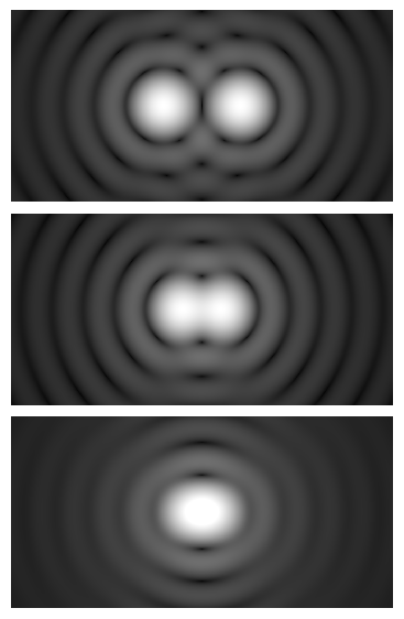
This image uses a nonlinear color scale (specifically, the fourth root) in order to better show the minima and maxima.
Artist: Spencer Bliven
Notice the numerical factor differs from Abbe’s expression. This is because Abbe’s and Rayleigh’s criteria address slightly different questions (grating resolution vs. point-source separation) and use different decision thresholds for “just resolved.” In practice, both formulas are used as rules-of-thumb. They deliver comparable scales and the same dependence on λ and NA. When quoting a resolution figure, it’s helpful to specify which convention you are using or simply state it as an approximate diffraction-limited resolution.
Coherence Matters: Incoherent vs. Coherent Illumination
Resolution limits also depend on the spatial coherence of illumination. In typical widefield brightfield and fluorescence imaging, illumination is designed to be spatially incoherent at the specimen (e.g., via Köhler illumination), yielding the conventional cutoff spatial frequency for incoherent imaging. Under fully coherent illumination (e.g., laser in certain configurations), the cutoff frequency changes, and the finest resolvable period scales differently with NA. Without diving deep into optical transfer mathematics, the practical advice is this:
- For standard brightfield and widefield fluorescence, the lateral resolution scales as ~
λ / (2·NA)to ~0.61·λ/NA. - For coherent systems, the resolving power depends on both the objective NA and the illumination NA (or equivalently condenser NA), and the cutoff differs. Matching condenser NA to objective NA is essential for brightfield to realize the incoherent limit.
Either way, diffraction enforces a boundary: below a certain feature size, contrast drops because those spatial frequencies are not transmitted to the image. For a given NA, you cannot “recover” these frequencies by increasing magnification alone. This is why discussions of empty magnification arise in microscopy education.
Axial Resolution and Sectioning
While most attention goes to lateral (x–y) resolution, the axial (z) dimension is equally important. The thickness of the focus, or optical section, also follows a diffraction scaling with NA. For widefield imaging, a common approximate expression for axial resolution is:
Δz (widefield) ~ 2 · n · λ / NA²where n is the refractive index of the imaging medium. This indicates axial resolution improves (i.e., the in-focus layer gets thinner) with higher NA and shorter wavelengths, and is also influenced by refractive index. Confocal and other sectioning techniques alter these relationships by attenuating out-of-focus light, but the underlying dependence of the PSF shape on NA remains. Later, in Depth of Field and Axial Resolution: How NA Controls Z, we contrast axial resolution with depth of field and focal tolerance from a practical viewpoint.
Key point: The “diffraction limit” is not one fixed number—it depends on what you are resolving (points vs. gratings), how you illuminate, and the system’s NA and wavelength. But all standard criteria reveal the same physics: higher NA and shorter wavelength support finer detail.
Magnification Myths, Empty Magnification, and Useful Range
Magnification enlarges the image but does not create detail. If the optical system cannot transmit higher spatial frequencies due to its NA, then increasing magnification simply spreads the same blur over more pixels or retinal area. This phenomenon is called empty magnification.
Useful Magnification and a Practical Rule-of-Thumb
A widely cited empirical guideline for visual observation is that the useful magnification range is approximately:
Useful visual magnification ≈ 500× to 1000× per NAFor instance, a 0.65 NA objective is typically most productive (by eye) at roughly 325× to 650×. Using 2000× with the same objective will not reveal additional fine structure; it will usually look dimmer and softer. While the exact limits vary with the observer’s eyesight, illumination, and contrast method, this range reflects the idea that image scale should match the optical information content.
For digital imaging, the concept translates to sampling. If the camera pixels are too large for the optical resolution at a given magnification (undersampling), fine details are not captured reliably. If the pixels are much smaller than required (oversampling), you will not gain resolution but may incur noise and storage penalties. Thus, rather than chasing headline magnification numbers, align total magnification with both NA and pixel size.
What Sets Apparent Sharpness at High Magnification?
Even before the strict diffraction limit is reached, several factors degrade sharpness as magnification increases:
- Numerical aperture: Ultimately defines the finest detail that can be transmitted with contrast.
- Aberrations: Spherical aberration from cover glass mismatch or immersion errors, field curvature, and chromatic aberrations all soften the image sooner at higher NA and magnification.
- Mechanical stability: Vibration and focus drift become more apparent at large magnification factors and shallow depth of field.
- Illumination and exposure: Higher magnification often lowers irradiance on the sensor or eye for a given NA, reducing signal-to-noise unless exposure or illumination is increased appropriately.
To prevent disappointment with “super magnification,” first ensure that NA is sufficient for the details you hope to see. Then verify that your system is well aligned (see Illumination, Coherence, and Condenser NA Matching), and that sampling is appropriate (see Camera Pixel Size, Sampling, and Nyquist in Microscopy).
Illumination, Coherence, and Condenser NA Matching
Illumination quality can either unlock the resolution allowed by your objective NA or leave it underutilized. In transmitted-light brightfield microscopy, two aspects are critical:

Images donated as part of a GLAM collaboration with Carl Zeiss Microscopy – please contact Andy Mabbett for details.
Artist: ZEISS Microscopy from Germany
- Spatial coherence and Köhler illumination: Köhler illumination uses conjugate planes to ensure even field illumination and to control the condenser aperture diaphragm independently from the field diaphragm. At the specimen, the illumination is effectively spatially incoherent, a condition that supports the well-known incoherent resolution limits.
- Condenser NA: The condenser focuses illumination into a cone defined by its aperture diaphragm, and its NA can be adjusted. For optimal brightfield resolution, the condenser NA should be similar to the objective NA (or modestly less to balance contrast and glare). If the condenser NA is too low, high-angle information is not illuminated, limiting contrast transfer at higher spatial frequencies.
Matching Condenser and Objective NA in Brightfield
In brightfield, the objective transfers image detail that has been encoded by the specimen’s interaction with the illumination field. If the illumination field lacks the necessary angular content, some spatial frequencies will not be excited, and the objective cannot image what was never illuminated. A practical approach is:
- For high-resolution brightfield work, set the condenser aperture diaphragm such that the effective illumination NA approaches the objective NA. This typically produces optimum resolution.
- If contrast is low or glare is problematic, slightly reduce the condenser NA to improve contrast at the cost of the very highest spatial frequencies.
Other contrast techniques have their own requirements. For instance, phase contrast and DIC use specialized condensers and optical elements to convert phase variations into intensity differences. These can approach the resolution of brightfield when properly adjusted but often involve their own balance between contrast and resolution. Darkfield requires a high-NA hollow cone of illumination that exceeds the objective’s NA, such that only scattered light enters the objective, emphasizing edges and small scatterers but with different resolution-contrast tradeoffs.
Illumination for Fluorescence
In widefield fluorescence, illumination is typically epi-illumination (through the objective) using a dichroic mirror to separate excitation and emission wavelengths. The concept of condenser NA does not apply in the same way; instead, the objective’s NA dictates both excitation cone (for epi-illumination) and emission collection. Resolution in widefield fluorescence follows the same scaling with λ and NA, but remember to use the emission wavelength in the diffraction limit expressions. The sampling guidance is often derived from the emission PSF.
Tip: Good illumination does not just mean “bright.” It means spatially uniform, appropriately incoherent for the modality, and with an aperture matched to the objective’s NA. This is the pathway to exploiting the resolution your optics are capable of.
Camera Pixel Size, Sampling, and Nyquist in Microscopy
Digital imaging introduces another resolution gate: sampling. Even if the optics produce a high-fidelity image at the intermediate image plane, the camera can only record detail down to the scale that its pixels sample. To preserve the information transmitted by the optics, sampling must satisfy the Nyquist criterion for the highest spatial frequencies present in the image.
From Optical Cutoff to Pixel Size
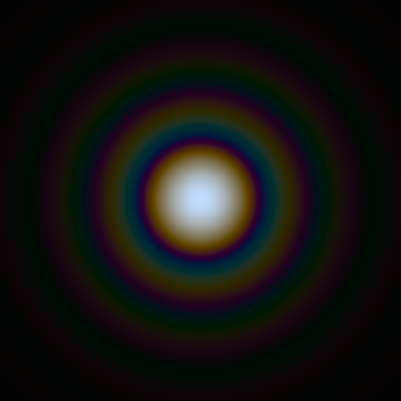
Artist: SiriusB
For incoherent imaging (typical of widefield brightfield and fluorescence), the optical transfer function (OTF) has a cutoff spatial frequency approximately given by:
f_c (incoherent) ≈ 2 · NA / λin object space. To sample this without aliasing, the sampling frequency should be at least twice the highest frequency, giving a sampling period:
p_sample ≤ 1 / (2 · f_c) ≈ λ / (4 · NA)Here, p_sample is the pixel size at the specimen. If your camera pixel pitch on the sensor is p_camera, and the total magnification from specimen to sensor is M_total, then:
p_sample = p_camera / M_totalRearranging gives a guide for selecting magnification relative to pixel pitch and NA:
M_total ≥ 4 · NA · p_camera / λIn practice, many microscopists target somewhere between λ/(3.3·NA) and λ/(4·NA) for p_sample to balance resolution preservation and signal-to-noise. For fluorescence, use emission wavelength for λ; for brightfield, a representative central wavelength (often ~550 nm) is used for estimation.
Calculating Effective Magnification to the Sensor
For finite-conjugate objectives (older designs), the objective magnification directly sets the image scale on the sensor if the optical path is designed accordingly. For modern infinity-corrected systems, the effective magnification is:
M_total = M_objective × (f_tube / f_reference) × M_camera_adapterwhere f_tube is the tube lens focal length in your microscope, and f_reference is the manufacturer’s reference tube lens focal length for which the objective magnification is specified (often 180 mm or 200 mm, depending on the brand). M_camera_adapter is the relay/c-mount adapter magnification to the camera sensor. If you are viewing by eye, the eyepiece can alter apparent angular magnification, but the resolving power remains governed by objective NA and the eye’s acuity.
Undersampling vs. Oversampling
- Undersampling: If
p_sampleis too large compared toλ/(4·NA), high-frequency details are not adequately captured and can alias, creating misleading patterns. Fine structures may appear as coarse or moiré-like artifacts. - Oversampling: If
p_sampleis much smaller than needed, images may look smoother but not sharper; the extra samples predominantly collect redundant information and read noise, potentially requiring longer exposure to achieve similar signal-to-noise. A mild degree of oversampling is quite common and safe; extreme oversampling offers diminishing returns.
Role of Deconvolution and Post-Processing
Computational techniques like deconvolution can redistribute contrast across spatial frequencies and improve apparent sharpness, especially in fluorescence imaging where a well-characterized PSF is available. However, deconvolution cannot conjure up spatial frequencies that were never recorded because of insufficient NA or gross undersampling. The output quality is fundamentally capped by the information content delivered by the optics and captured according to Nyquist.
Align your acquisition planning with the optics: if your objective has NA 1.4 for green fluorescence, choose camera pixel size and magnification so that Nyquist is met for the emission wavelength, not for blue or red unless you image those channels as well. This ensures each channel is sampled adequately for its resolution potential.
Depth of Field and Axial Resolution: How NA Controls Z
Two related but distinct concepts describe sharpness along the optical axis: axial resolution and depth of field (DOF). Axial resolution concerns the smallest separation along z at which two features can be distinguished, whereas DOF is the axial range over which a single feature appears acceptably focused.
Axial Resolution Scaling
As introduced in Optical Resolution Limits, a widely used approximation for widefield axial resolution is:
Δz ~ 2 · n · λ / NA²
Artist: Anaqreon
This scaling highlights the power of high NA for optical sectioning. Doubling NA reduces the axial PSF extent by a factor of four, dramatically thinning the in-focus slice. This is why high-NA oil objectives often give crisp detail but can be unforgiving of focus drift.
Depth of Field Considerations
DOF is influenced by diffraction and by the imaging system’s acceptance of slight defocus. For a diffraction-limited system, a common approximation for the diffraction component of DOF scales as:
DOF (diffraction-limited) ∝ λ · n / NA²Additional terms can arise from sensor pixel size or the observer’s visual acuity (often captured as a “circle of confusion” in geometric optics), further increasing the acceptable DOF. Practically, higher NA reduces DOF, making it easier to isolate thin features but requiring steadier focusing and often thinner specimens or optical sectioning methods for thick samples.
Implications for Thick and Heterogeneous Samples
In thick specimens, refractive index variations and scattering can broaden the effective PSF and reduce both axial and lateral resolution, especially at high NA. Using immersion media that better match the specimen’s refractive index can reduce spherical aberration, as discussed in Immersion Media: Air, Water, and Oil Objectives. For very thick or scattering samples, techniques beyond widefield (e.g., confocal, light-sheet, or multiphoton) may be preferred for improved axial sectioning and contrast.
Summary: High NA sharpens details in x–y and thins the focal slice in z. The trade-off is reduced depth of field and greater sensitivity to alignment and refractive index matching.
Immersion Media: Air, Water, and Oil Objectives
The refractive index of the medium between the specimen and the objective front lens directly enters the NA definition (NA = n · sin θ). Changing the medium changes both the achievable NA and the optical aberrations encountered when imaging through a cover glass and into a specimen. Three common categories are:
Air Objectives
- Refractive index: n ≈ 1.00.
- Typical NA range: up to ~0.95 for high-performance air objectives.
- Use cases: Convenient for general observation, dry specimens, or when immersion media are impractical.
- Trade-offs: Limited maximum NA; more susceptible to refractive index mismatch when imaging into aqueous specimens covered by standard cover glasses.
Water-Immersion Objectives
- Refractive index: n ≈ 1.33.
- Typical NA range: ≈ 1.0–1.2 for many designs.
- Use cases: Imaging live cells and aqueous environments where refractive index matching reduces spherical aberration compared to air objectives.
- Trade-offs: Water can evaporate and requires more frequent replenishment; some designs include correction collars to handle cover glass variations.
Oil-Immersion Objectives
- Refractive index: n ≈ 1.515 for many microscope immersion oils (matched to standard cover glasses).
- Typical NA range: ≈ 1.25–1.45.
- Use cases: Maximizing resolution with high NA for thin specimens mounted under standard cover glasses.
- Trade-offs: Requires careful handling to avoid contamination; sensitive to cover glass thickness (often specified as 0.17 mm, No. 1.5) and to using the correct oil type for the objective design.
Cover Glass Thickness and Correction
High-NA objectives are commonly corrected for a specific cover glass thickness, typically around 0.17 mm (No. 1.5). Deviations in thickness or refractive index can introduce spherical aberration, reducing contrast and effective resolution. Some objectives provide a correction collar that allows the user to compensate for small variations. The higher the NA, the more critical it is to adhere to the specified coverslip and immersion conditions to realize the promised resolution.
When choosing immersion media, consider the sample’s environment. Water immersion is a good match for live, aqueous specimens, minimizing refractive index mismatch across interfaces and reducing axial aberrations. Oil immersion favors maximum NA and resolution but is best suited for thin, well-mounted specimens under standard cover glasses. There is no universally “best” immersion; the right choice follows your sample’s optical path and your resolution goals.
Common Misconceptions and How to Check Your Optics
Discussions of NA, resolution, and magnification are fertile ground for myths. Clearing up these misconceptions can save time and guide better choices.
Misconception 1: “Higher Magnification Always Means Higher Resolution”
It does not. Magnification without sufficient NA produces larger, blurrier images—a classic case of empty magnification. If you find yourself cranking up magnification to “see more detail” but the image gets softer, you have likely exceeded the useful range for your objective’s NA and your camera’s sampling.
Misconception 2: “Resolution Is One Number”
Resolution depends on your specimen, imaging modality, wavelength, and even your definition (Abbe vs. Rayleigh). It’s more accurate to speak of diffraction-limited lateral resolution and axial resolution, and to be clear about the imaging modality and wavelength assumptions. See Optical Resolution Limits for context.
Misconception 3: “I Can Bypass NA Limits with Post-Processing”
Computational sharpening can redistribute contrast, but it cannot reliably restore frequencies that never reached the sensor due to insufficient NA or undersampling. Deconvolution works best when imaging is near diffraction-limited and the PSF is known; it is not a substitute for inadequate optics.
Misconception 4: “All High-NA Objectives Are the Same”
Objectives differ in aberration correction, field flatness, chromatic performance, working distance, and sensitivity to cover glass variations. Two objectives with the same NA can deliver different contrast and edge sharpness due to these aberrations and coatings. Always align expectations with the objective class and your specimen preparation.
Checking Your Optical Performance
You can qualitatively assess whether your system is close to its expected performance with simple observations and test targets:
- Use a fine periodic target: For brightfield, a high-quality ruled grating or resolution test slide helps reveal whether contrast persists near the expected cutoff for your NA and wavelength.
- Adjust the condenser aperture: If fine detail improves as you open the condenser iris to match the objective NA, your illumination was previously starved of high-angle components. See Illumination, Coherence, and Condenser NA Matching.
- Check coverslip and immersion: With high-NA immersion objectives, verify correct coverslip thickness and immersion medium. Improvements in contrast and sharpness after correcting these indicate prior spherical aberration.
- Inspect sampling: If you suspect undersampling, increase
M_total(e.g., use a higher objective magnification or different camera adapter) and check whether fine detail is recovered without aliasing. Refer back to Camera Pixel Size, Sampling, and Nyquist.
These sanity checks are educational and can guide refinements, keeping the process strictly observational and non-invasive, consistent with good microscopy practice.
Frequently Asked Questions
Does 1000× always resolve bacteria?
No. Resolving small bacteria depends primarily on NA and wavelength, not on headline magnification. Many bacteria are about 0.5–1.0 µm in width, which is near or below the lateral resolution limit of lower-NA objectives. A high-NA oil objective (e.g., NA ≈ 1.3–1.4) under suitable illumination can resolve submicron features better than a low-NA objective at the same or even higher magnification. If the optics cannot transmit the necessary spatial frequencies (see Abbe and Rayleigh criteria), increasing magnification alone won’t help; it only enlarges the diffraction blur.
Is a 4K camera always better for microscopy resolution?
Not necessarily. A 4K camera has more pixels, but if the pixel size and total magnification do not satisfy Nyquist sampling relative to your objective’s NA and wavelength, the extra pixels may not translate into higher resolvable detail. The key is matching pixel size at the specimen to the optical resolution limit. A well-matched lower-resolution camera can outperform a mismatched higher-resolution sensor in terms of actual captured detail and signal-to-noise ratio.
Final Thoughts on Choosing the Right NA and Magnification
At the heart of every sharp micrograph lies a simple physics story: light is a wave, and lenses inevitably diffract it. Numerical aperture is how a microscope objective “leans into” that wave nature, gathering high-angle light that encodes fine spatial detail. Magnification then presents that information at a useful scale for your eye or camera—but only if the information exists to begin with. The practical consequences are consistent across brightfield and fluorescence:

Artist: Happie1Soul
- Prioritize NA for resolution: Higher NA supports finer detail and thinner optical sections. Choose immersion media and cover glass conditions that suit your specimen to control aberrations (see Immersion Media).
- Match illumination to the optics: Properly adjusted Köhler illumination and condenser aperture (for brightfield) help realize the incoherent resolution limits.
- Align magnification with sampling: Select objective/adapters and cameras so that pixel size at the specimen meets Nyquist for your NA and wavelength. Avoid both obvious undersampling and gratuitous oversampling.
- Mind depth of field and axial resolution: Higher NA reduces DOF and enhances axial resolving power. Plan focus stability and consider optical sectioning methods for thick or scattering samples (see Depth of Field and Axial Resolution).
- Verify performance empirically: Simple test patterns, condenser adjustments, and checks on immersion/coverslip conditions can confirm you are near the diffraction-limited behavior of your system (see Common Misconceptions and How to Check Your Optics).
By making NA the central criterion—then tuning illumination, magnification, and sampling accordingly—you can consistently approach the true resolving power of your microscope. If this article clarified concepts you’ve wondered about, consider subscribing to our newsletter. You’ll receive future deep dives into microscope fundamentals, comparisons of imaging modalities, and practical guides for optimizing your system’s optical performance—always with a focus on accurate physics, clear explanations, and actionable insight.

