Table of Contents
- What Determines Resolution in Optical Microscopy?
- Magnification vs. Resolution: Clearing the Confusion
- Numerical Aperture Explained: Light-Gathering and Angular Range
- Abbe and Rayleigh Criteria: Practical Resolution Limits
- Axial Resolution, Depth of Field, and Refractive Index
- Wavelength and Illumination: Color, Monochrome, and Coherence
- Sampling, Nyquist, and Camera Pixel Size
- Immersion Media and Refractive Index Matching
- Aberrations, Coverslips, and Alignment
- Contrast Mechanisms and Their Resolution Trade-offs
- Practical Calculations: From NA and Wavelength to Resolution
- Common Misconceptions About Resolution
- Frequently Asked Questions
- Final Thoughts on Choosing the Right Resolution Strategy
What Determines Resolution in Optical Microscopy?
In optical microscopy, resolution is the smallest distance between two points that can still be distinguished as separate. It is not the same as magnification, and it is not set by the number of pixels in your camera alone. Resolution emerges from a combination of optical physics, illumination, detection, and sample properties. Appreciating how these factors interact helps you choose objectives, illumination, and acquisition settings that actually improve the visibility of fine detail—rather than just producing larger images.
The core parameters that govern resolution include:
- Numerical aperture (NA): A measure of the objective’s light-gathering ability and angular acceptance. NA appears directly in most resolution formulas.
- Wavelength (λ): Shorter wavelengths support finer spatial detail; resolution scales approximately with λ/NA.
- Refractive index (n): The immersion medium’s refractive index sets the upper bound on NA and influences axial resolution and aberrations.
- Illumination coherence and geometry: In incoherent widefield imaging (e.g., fluorescence), the optical transfer function has a different cutoff than in coherent or partially coherent brightfield, changing effective resolution constants.
- Sampling (pixels and scanning steps): The detector must sample at or above the Nyquist rate to capture the finest spatial frequencies delivered by the optics.
- Aberrations and alignment: Spherical and chromatic aberrations, as well as imperfect coverslip and condenser alignment, can degrade the contrast of high spatial frequencies.
By analyzing these elements together, you can predict when changing objectives, switching immersion media, or adjusting camera magnification will yield a real increase in resolvable detail. The sections below break down each factor, with practical formulas and examples you can use immediately.
Magnification vs. Resolution: Clearing the Confusion
Magnification makes features look larger, but resolution makes features distinct. This difference is foundational:
- Magnification is the ratio between an object’s apparent size in the image and its actual size. Optical magnification arises primarily from the objective and tube lens; digital magnification (or digital zoom) simply resamples or enlarges pixels.
- Resolution is the smallest separation at which two features can be distinguished as separate. It depends on NA, wavelength, aberrations, and sampling—not on how large the image appears.
As a result:
- Increasing optical magnification beyond what your objective’s NA and your detector’s sampling can support leads to empty magnification: bigger pixels, no new detail.
- A modest increase in NA or a shorter wavelength can yield a true increase in resolvable detail, even if magnification remains unchanged.
- Matching magnification to pixel size and optical cutoff avoids undersampling and makes full use of your objective’s resolving power.
An effective workflow starts with the optical resolution limit set by NA and wavelength, then chooses magnification so that the camera samples those finest details at or above the Nyquist criterion.
Numerical Aperture Explained: Light-Gathering and Angular Range
Numerical aperture is defined by NA = n · sin(θ), where n is the refractive index of the medium between the objective front lens and the specimen (air, water, glycerol, or oil), and θ is half the angular aperture of the objective. NA influences both resolution and brightness:

- Higher NA captures higher-angle diffracted light, which encodes fine spatial detail. This is why NA appears in the denominator of resolution formulas.
- Higher NA also increases the cone of collected light, boosting signal and contrast for high spatial frequencies.
A few practical notes:
- Upper bounds: In air (
n ≈ 1.0), maximum usable NA is close to 0.95 for dry objectives becausesin(θ) ≤ 1. Using immersion media withn > 1allows NA above 1.0 (e.g., oil immersion NA ≈ 1.3–1.49). - Immersion matching: The specified NA assumes the objective is used with its intended immersion medium and coverslip thickness. Mismatches reduce effective resolution through aberrations.
- Illumination dependence: In transmission modalities, condenser NA and its alignment also matter. In fluorescence, objective NA dominates collection; illumination NA affects excitation distribution but not the emission collection cutoff.
Because NA links directly to the acceptance of high-angle diffracted orders, it is the primary lever for improving optical resolution—subject to careful control of immersion conditions and aberrations.
Abbe and Rayleigh Criteria: Practical Resolution Limits
Optical resolution limits can be quantified in several closely related ways. Two commonly used expressions are the Abbe limit for periodic features and the Rayleigh criterion for point-like emitters.
Abbe limit (periodic structures)
For incoherent widefield imaging, the highest spatial frequency transmitted by the system is set by the optical transfer function cutoff. For a sinusoidal grating or periodic structure, Abbe’s criterion states the minimum resolvable period d is approximately:
d ≈ λ / (2 · NA)
Here, λ is the relevant imaging wavelength and NA is the objective’s numerical aperture on the detection side. This formulation reflects the need to capture at least the zero and first diffracted orders to reconstruct the periodic detail.
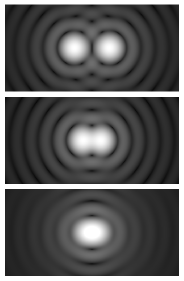
Rayleigh criterion (point-like emitters)
For two point sources imaged incoherently (such as two closely spaced fluorescent emitters), the Rayleigh criterion defines the distance r at which the principal maximum of one point spread function (PSF) coincides with the first minimum of the other:
r ≈ 0.61 · λ / NA
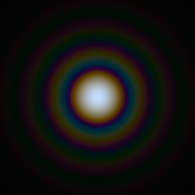
This image uses a nonlinear color scale (specifically, the fourth root) in order to better show the minima and maxima. — Artist: Spencer Bliven
This expression captures a similar scaling with λ/NA, with a constant that reflects the shape of the Airy pattern in incoherent imaging. The 0.61 factor corresponds to the first zero of the Bessel function that describes the Airy disk intensity distribution.
Optical transfer function (OTF) perspective
It is often useful to think in frequency space. The incoherent OTF has a cutoff spatial frequency:
f_c (incoherent) = 2 · NA / λ(cycles per unit length)
For coherent imaging of amplitude objects, the cutoff is lower:
f_c (coherent) = NA / λ
These expressions explain why brightfield performance depends on illumination coherence and condenser settings, while fluorescence resolution typically follows the incoherent model dominated by emission wavelength and collection NA. In all cases, higher NA and shorter wavelengths push the cutoff to higher spatial frequencies, supporting finer detail.

Every other practical factor—focus quality, aberrations, sampling—affects how close you can get to these limits in real images by shaping the PSF or attenuating high spatial frequencies.
Axial Resolution, Depth of Field, and Refractive Index
Resolution is three-dimensional. Lateral resolution (in the focal plane) is commonly quoted using Abbe or Rayleigh expressions, but axial (z) resolution and depth of field (DOF) are equally important for thick specimens and optical sectioning.
Axial resolution (widefield, approximate)
For incoherent widefield imaging, a widely used approximation for axial resolution is:
Δz (axial) ≈ 2 · n · λ / NA²
Here n is the refractive index of the imaging medium, and λ is the emission or imaging wavelength. This approximation captures the strong dependence on NA squared: increasing NA substantially improves axial discrimination. It also reflects that higher refractive index media reduce the axial spread of the PSF.
Depth of field
Depth of field is the axial range over which features remain acceptably sharp in the image. DOF includes a diffraction (wave) term and a geometric term related to pixel size and magnification. A common approximation for the diffraction-limited contribution is:
DOF_wave ≈ n · λ / NA²
The geometric term depends on the acceptable blur on the detector. One useful way to think about it is that larger pixels or lower magnification tolerate more defocus before blur spans multiple pixels. The exact formula you use will depend on your definition of acceptable sharpness and your camera’s pixel size; the main takeaway is that both wave optics and imaging geometry contribute to DOF.
Refractive index and axial scaling
Imaging through media with refractive indices different from the immersion medium can change apparent axial distances (axial scaling) and introduce spherical aberration. When imaging deep into samples, matching refractive indices as closely as practical and limiting refractive index discontinuities helps maintain both lateral and axial resolution.
While the formulas above are approximations, they provide reliable guidance for planning z-step spacing, interpreting axial detail, and understanding why high-NA immersion objectives offer improved sectioning capability compared with lower-NA dry objectives.
Wavelength and Illumination: Color, Monochrome, and Coherence
Wavelength appears explicitly in every resolution expression, but selecting wavelengths is often constrained by your sample’s properties, dyes, and illumination source. Here are the key considerations:
- Shorter wavelengths improve resolution: All else equal, using a shorter imaging wavelength reduces
λ/NAand therefore the diffraction-limited spot size. In fluorescence, the relevant λ is typically the emission wavelength band used for detection. - Monochromatic vs. polychromatic light: Broad spectral bands produce a range of PSF sizes and can introduce chromatic aberration if not corrected by the objective. Narrower detection bands reduce dispersion and help maintain consistent resolution across the image.
- Coherence and modality: In incoherent fluorescence imaging, resolution follows the incoherent OTF with
f_c = 2 · NA / λ. In brightfield or phase-contrast imaging, the degree of spatial coherence (affected by condenser NA and aperture settings) influences contrast and the effective bandwidth of transferred spatial frequencies. - Photon budget: Shorter wavelengths can increase photobleaching or scattering; evaluate trade-offs rather than defaulting to the shortest possible λ.
Optimizing illumination is not only about color; it also involves proper condenser adjustment. Although this article focuses on detection-side resolution, correct brightfield illumination (e.g., Köhler) ensures even field, appropriate coherence, and improved contrast—indirectly supporting your ability to realize the theoretical limits.
Sampling, Nyquist, and Camera Pixel Size

Optics can deliver high spatial frequencies, but your detector must sample them adequately. The Nyquist–Shannon sampling theorem states that to reconstruct a band-limited signal, you must sample at least twice the highest frequency present. In microscopy, that highest frequency is the OTF cutoff.
Sampling for incoherent widefield imaging
For incoherent imaging with cutoff f_c = 2 · NA / λ, the sampling interval at the specimen (the effective pixel size in object space) should satisfy:
p_object ≤ 1 / (2 · f_c) = λ / (4 · NA)
This simple expression connects optics and camera directly. The effective pixel size at the specimen plane is:
p_object = p_sensor / M
where p_sensor is the camera pixel pitch and M is the total optical magnification between the sample and sensor. Combining the two:
p_sensor / M ≤ λ / (4 · NA)→ chooseMso thatp_objectmeets or beats this bound.
For example, with 6.5 µm pixels and green light (λ ≈ 550 nm) at NA 1.40, λ/(4·NA) ≈ 98 nm. You would want p_object ≤ 98 nm, implying M ≥ 6.5 µm / 0.098 µm ≈ 66×.
Undersampling and oversampling
- Undersampling (pixels too large for the optical cutoff) causes aliasing: high spatial frequencies masquerade as lower ones, creating false patterns and losing real detail.
- Oversampling (pixels much smaller than needed) does not recover more optical detail but can help with sub-pixel localization and deconvolution at the cost of larger files and lower per-pixel signal-to-noise.
Line scanners and step sizes
The same Nyquist logic applies to scanning systems: stage step sizes or beam scanning increments should be ≤ λ / (4 · NA) for incoherent imaging if you wish to sample the lateral resolution limit fully. In z-stacks, a common planning rule is to sample axial steps at half of the estimated axial resolution—see axial approximations—to avoid missing details in depth.
Matching pixel size and step spacing to the optical bandwidth is one of the most impactful and accessible ways to unlock resolution you may already have in your system.
Immersion Media and Refractive Index Matching
Because NA = n · sin(θ), raising the refractive index n via immersion increases the ceiling on NA and typically improves resolution, brightness, and contrast of fine detail. The commonly used immersion options include:
- Air (n ≈ 1.00): Convenient and clean, but limits NA to ≲ 0.95 and is sensitive to refractive index mismatch when imaging through thick aqueous samples.
- Water (n ≈ 1.33): Well matched to live biological specimens and aqueous media; enables high NA without large index mismatches at shallow to moderate depths.
- Glycerol (n ≈ 1.47): A compromise between water and oil; useful when samples or mounting media have intermediate refractive indices.
- Oil (n ≈ 1.515, typical microscope immersion oils): Supports very high NA objectives (≈ 1.3–1.49). Best for thin, well-mounted specimens on standard coverslips with matching refractive indices.
Considerations when choosing immersion:
- Index matching: Using an immersion medium whose refractive index closely matches the sample or mounting medium minimizes spherical aberration and preserves axial resolution.
- Coverslip thickness: Many high-NA objectives are corrected for #1.5H coverslips (≈ 0.17 mm). Deviations can introduce aberrations; some objectives include a correction collar to compensate for thickness and temperature-induced index changes.
- Working distance: High-NA immersion objectives often have short working distances; ensure your specimen geometry is compatible.
When used as designed—with the correct coverslip and immersion medium—high-NA objectives deliver the lateral and axial performance predicted by the Abbe and Rayleigh limits. Improper use can forfeit much of that theoretical advantage.
Aberrations, Coverslips, and Alignment
Even with optimal NA and wavelength, aberrations can reduce high-frequency contrast and broaden the PSF. Common contributors include:
- Spherical aberration: Arises from refractive index mismatch or incorrect coverslip thickness. It blurs focus, particularly along the optical axis, and reduces both lateral and axial resolution.
- Chromatic aberration: Wavelength-dependent focus shift or magnification changes. Apochromatic objectives correct these effects over specified spectral ranges; using emission filters within those ranges helps maintain performance.
- Coma and astigmatism: Off-axis aberrations that distort point images away from the center of the field; more relevant in wide fields or when objectives are used off-design.
- Field curvature and distortion: Curved best-focus surface or non-linear magnification. These do not necessarily reduce on-axis resolution but affect uniformity across the image.
Practical steps to limit aberrations:
- Use the intended coverslip: For high-NA imaging, a #1.5H coverslip of 0.17 mm nominal thickness is often specified. Check the objective engraving and datasheet.
- Adjust correction collars: If present, they allow fine compensation for coverslip thickness and temperature-induced index changes. Small adjustments can noticeably improve sharpness.
- Align illumination: In brightfield, proper condenser and aperture alignment (e.g., Köhler illumination) reduces glare, ensures even field, and supports the desired coherence for contrast. See illumination considerations.
- Stabilize temperature and index: Large temperature differences can shift refractive indices and coverslip thicknesses slightly; allow the system to equilibrate.
Many aberrations scale with NA; the higher the NA, the more sensitive your system becomes to small deviations from design conditions. That is a strong argument for paying attention to the seemingly mundane details like coverslip quality and alignment when you invest in high-NA imaging.
Contrast Mechanisms and Their Resolution Trade-offs
Different contrast mechanisms interact with resolution in distinct ways. While the diffraction limit remains fundamental, practical resolution—the smallest features you can see with adequate contrast—depends on modality.
- Brightfield (transmitted light): Contrast arises from absorption and scattering. Effective resolution depends on illumination coherence and condenser settings; stopping down the condenser improves contrast for low-contrast specimens but reduces high-frequency transfer.
- Phase contrast: Converts phase shifts into intensity differences. It enhances visibility of transparent structures but can introduce halos that complicate interpretation of fine boundaries.
- Differential interference contrast (DIC): Provides gradient-based contrast, excellent for edges and subtle relief. DIC can make fine details more apparent but renders absolute intensities nonlinearly.
- Polarization contrast: Sensitive to birefringence; resolution follows basic optical constraints but contrast depends on specimen anisotropy.
- Fluorescence (widefield): Incoherent emission imaging; resolution follows Abbe/Rayleigh with emission wavelength and collection NA. Optical sectioning is limited without additional techniques.
- Confocal fluorescence: A pinhole rejects out-of-focus light, improving contrast and axial sectioning; lateral resolution can be modestly improved with small pinholes. Sampling and pinhole size should be chosen to balance signal and resolution.
- Structured illumination and deconvolution (linear methods): Computational approaches can restore high-frequency contrast attenuated by the OTF. Deconvolution is most effective when data are well-sampled and the PSF is known or well-estimated.
Choosing a contrast mechanism is a trade-off among resolution, sectioning, speed, and photophysics. Regardless of modality, the best results come from harmonizing NA, wavelength, and sampling with the modality’s strengths.
Practical Calculations: From NA and Wavelength to Resolution
The formulas above become most useful when applied to real imaging scenarios. The following worked examples illustrate how to translate NA and wavelength into lateral resolution, sampling requirements, and approximate axial performance for incoherent widefield imaging.
Example 1: Air objective, moderate NA
- Objective: 40× air, NA = 0.65
- Imaging wavelength: λ = 550 nm (green)
- Camera pixel: p_sensor = 6.5 µm
Resolution estimates:
- Rayleigh (points):
r ≈ 0.61 · λ / NA = 0.61 · 550 nm / 0.65 ≈ 516 nm - Abbe (periodic):
d ≈ λ / (2 · NA) = 550 nm / 1.30 ≈ 423 nm
Sampling requirement (Nyquist for incoherent imaging):
- Specimen sampling interval:
p_object ≤ λ / (4 · NA) = 550 nm / 2.6 ≈ 212 nm - Minimum magnification for 6.5 µm pixels:
M ≥ p_sensor / p_object ≈ 6.5 µm / 0.212 µm ≈ 31×
Since the optical magnification is 40×, the effective object-space pixel is 6.5 µm / 40 ≈ 162.5 nm, which meets the Nyquist criterion (162.5 nm < 212 nm). The camera can sample the optical resolution of this objective at λ ≈ 550 nm without aliasing.
Axial scale (approximate):
- Axial resolution:
Δz ≈ 2 · n · λ / NA²withn = 1.0givesΔz ≈ 2 · 0.55 µm / 0.65² ≈ 2.60 µm. - Wave DOF contribution:
DOF_wave ≈ n · λ / NA² ≈ 1.30 µm.
Interpretation: Lateral details near ~0.5 µm are resolvable with adequate contrast; the camera sampling is sufficient, and axial discrimination is on the order of a few micrometers in air.
Example 2: High-NA oil immersion
- Objective: 60× oil, NA = 1.40
- Imaging wavelength: λ = 550 nm
- Immersion oil: n ≈ 1.515
- Camera pixel: p_sensor = 6.5 µm
Resolution estimates:
- Rayleigh (points):
r ≈ 0.61 · 550 nm / 1.40 ≈ 240 nm - Abbe (periodic):
d ≈ 550 nm / (2.8) ≈ 196 nm
Sampling requirement:
- Specimen sampling interval:
p_object ≤ 550 nm / (4 · 1.40) ≈ 98 nm - Minimum magnification for 6.5 µm pixels:
M ≥ 6.5 µm / 0.098 µm ≈ 66×
At 60×, p_object ≈ 6.5 µm / 60 ≈ 108 nm, which is slightly larger than the Nyquist target for λ = 550 nm. This is close in practice; increasing magnification to ~100× would comfortably satisfy Nyquist in this spectral band with 6.5 µm pixels.
Axial scale (approximate):
- Axial resolution:
Δz ≈ 2 · n · λ / NA² ≈ 2 · 1.515 · 0.55 µm / 1.40² ≈ 0.85 µm - Wave DOF contribution:
DOF_wave ≈ 1.515 · 0.55 µm / 1.40² ≈ 0.43 µm
Interpretation: High NA and oil immersion deliver sub-250 nm lateral Rayleigh separations in green light, with sub-micrometer axial resolution in widefield. Sampling should be chosen to avoid undersampling of the highest spatial frequencies.
Example 3: Choosing wavelength and sampling together
- Objective: 100× oil, NA = 1.45
- Imaging wavelength options: λ = 488 nm (blue-green), 561 nm (yellow-green)
- Camera: 4.5 µm pixels
Nyquist sampling intervals:
- At 488 nm:
λ/(4·NA) ≈ 488 nm / (4 · 1.45) ≈ 84 nm; with 100×,p_object = 4.5 µm / 100 = 45 nm(oversampled) - At 561 nm:
561 nm / (4 · 1.45) ≈ 97 nm; with 100×,p_object = 45 nm(oversampled)
With smaller pixels and high magnification, both wavelengths are well-sampled. Blue-green light supports finer optical resolution, but practical choices may also be guided by fluorophore performance and sample photostability. Oversampling increases data size but can assist with deconvolution.
Putting it together
These calculations provide actionable decisions:
- Estimate optical resolution using Abbe or Rayleigh.
- Set camera magnification so Nyquist is met for the wavelength band you will detect.
- Choose immersion and coverslip standards to minimize aberrations.
- Confirm contrast modality supports visibility of your target features without overly restricting high-frequency transfer.
Common Misconceptions About Resolution
Resolution discussions often get tangled in myths. Here are frequent misconceptions and the corresponding clarifications grounded in optical theory:
- “More magnification always reveals more detail.”
False when optics or sampling are limiting. Beyond the optical and sampling limits, higher magnification just produces larger, blurrier pixels—empty magnification. - “Higher megapixel cameras guarantee higher resolution.”
Not necessarily. Pixel count increases field of view at fixed sampling, but pixel size relative to magnification determines whether the camera can capture the available optical detail. - “NA only affects brightness, not resolution.”
Incorrect. NA directly sets the angular range of captured diffracted light and appears in the denominator of the resolution formulas. Higher NA improves both brightness and resolvable detail. - “Shorter wavelength is always better.”
Shorter λ improves resolution, but may increase photodamage, scattering, or be incompatible with your labels. Balance λ with contrast, sample viability, and signal-to-noise. - “Closing the condenser aperture always improves the image.”
It may boost low-frequency contrast in brightfield but reduces high-frequency transfer and can lower resolution for fine detail. Adjust for the specimen and modality. - “Digital zoom is equivalent to optical magnification.”
Digital zoom resamples the image and cannot add optical detail absent from the acquisition. Use optical magnification and proper sampling to capture real detail at the outset. - “Any coverslip will do.”
High-NA imaging is sensitive to coverslip thickness and refractive index. Using the specified #1.5H (≈ 0.17 mm) coverslip and setting the correction collar, if available, can noticeably improve resolution.
Frequently Asked Questions
Is resolution the same as pixel size?
No. Pixel size determines how finely you sample the image formed by the optics, but the optical system sets the finest detail that exists in that image. To capture all the detail available from the objective, the effective pixel size at the specimen should meet the Nyquist criterion based on the optical cutoff. If pixels are larger than this, you lose detail to undersampling; if they are much smaller, you gain file size without adding optical resolution, though oversampling can help some analyses.
Why do my images look soft with high-NA oil objectives?
Common reasons include refractive index mismatch or incorrect coverslip thickness, which cause spherical aberration; slight misfocus due to the shallower depth of field at high NA; and undersampling when magnification and pixel size do not meet Nyquist. Check that you are using the intended immersion oil, a #1.5H coverslip around 0.17 mm, and, if the objective has a correction collar, adjust it carefully. Also ensure your camera sampling is appropriate for the objective and wavelength.
Final Thoughts on Choosing the Right Resolution Strategy

Microscope resolution is governed by a concise set of physical relationships: detail scales with λ/NA, and capturing that detail depends on sampling at or above Nyquist while minimizing aberrations. The most effective path to sharper, more informative images is to harmonize four pillars:
- Optics: Choose NA suitable for your feature scales and specimen geometry. Use the correct immersion medium and coverslip to preserve the designed performance.
- Wavelength: Select detection bands that balance resolution with brightness and specimen needs.
- Sampling: Set magnification and pixel size to satisfy Nyquist for the optical cutoff at your chosen wavelength.
- Alignment and aberration control: Maintain proper illumination, adjust correction collars when available, and keep the system mechanically and thermally stable.
When these elements are in tune, improvements in image sharpness are not just subjective—they are supported by theory and evident in measurable features. Use the formulas and checklists in this article as a planning guide whenever you switch objectives, change emission filters, or evaluate a new camera. If you found this deep dive helpful, explore our related fundamentals articles and subscribe to our newsletter to receive future installments on optics, sampling, and contrast methods.

