Table of Contents
- What Is Numerical Aperture (NA) and Why It Controls Resolution?
- How Resolution, Magnification, and Pixel Sampling Interact
- Illumination Geometry and Contrast: Köhler vs Critical
- The Condenser’s Role: Matching NA and Using the Aperture Diaphragm
- Depth of Field, Working Distance, and NA Trade-offs
- Refractive Index, Immersion Media, and Spherical Aberration
- Wavelength Choice, Color, and Chromatic Effects
- Quantifying Resolution: Abbe, Rayleigh, Sparrow, and MTF
- Calibrating Field of View and Avoiding Empty Magnification
- Frequently Asked Questions
- Final Thoughts on Choosing the Right Numerical Aperture and Illumination Strategy
What Is Numerical Aperture (NA) and Why It Controls Resolution?
Numerical aperture (NA) is a cornerstone parameter in optical microscopy. It quantifies the light-gathering ability and angular acceptance of an optical element, such as a microscope objective or condenser. In object space, it is defined as NA = n sin(θ), where n is the refractive index of the medium between the specimen and the objective’s front lens (air, water, or immersion oil), and θ is half the angular extent of the light cone that the objective accepts from the specimen. A higher NA implies a wider acceptance angle and, therefore, a greater ability to collect high-angle diffracted light that carries fine spatial detail.
Why does this matter? Because spatial resolution—the ability to distinguish small, closely spaced features—depends fundamentally on diffraction. When light from a point or a fine detail passes through a lens, it does not form a perfect point but a diffraction pattern. The extent of this pattern sets a limit on how close two points can be while still being resolved as separate.
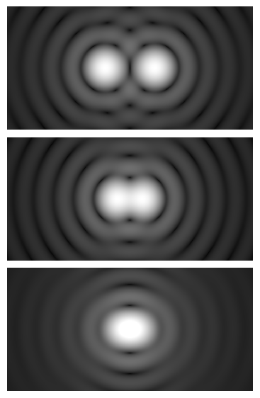
Two widely cited criteria for lateral (x–y) resolution in incoherent widefield imaging are:
- Rayleigh Criterion: The minimum resolvable distance
d_R ≈ 0.61 λ / NA, where λ is the wavelength in the medium (often approximated by the wavelength in air divided by the medium’s refractive index for practical purposes). This criterion is based on the first minimum of one point’s diffraction pattern coinciding with the maximum of the other. - Abbe Limit (in an incoherent imaging context): Often invoked as a similar order-of-magnitude limit, with a common expression for periodic structures under incoherent illumination related to the objective’s NA as well. In practical, modern widefield microscopy, the Rayleigh-based estimate
∼0.61 λ / NAis a useful rule of thumb.
Artist: Spencer Bliven
Axial (z) resolution is typically poorer than lateral resolution in widefield systems. A commonly used scaling relation is that axial resolution degrades roughly with 1 / NA². A simplified estimate for widefield axial resolution depends on the refractive index and NA, highlighting again that higher NA not only improves lateral detail but also tightens the depth response.
It is crucial to emphasize that magnification alone does not determine resolution. Magnification simply scales the image. If optical resolution is limited by NA and wavelength, increasing magnification beyond a certain point does not reveal new detail—it only makes the same blurred pattern larger. This is a classic pitfall known as empty magnification (see Calibrating Field of View and Avoiding Empty Magnification).
Two related concepts that interact with NA are contrast and signal-to-noise ratio (SNR). While resolution describes the system’s ability to capture high spatial frequencies, contrast determines how visible those details are against background intensity variations. Illumination geometry, condenser settings, and sample properties all influence contrast. You will see how these elements tie together when we examine Köhler illumination and the condenser aperture.
How Resolution, Magnification, and Pixel Sampling Interact
Modern microscopy frequently involves digital imaging. That adds a key consideration: sampling. To represent an optical image faithfully, the camera’s pixel grid must sample the image at a rate sufficient to capture the finest spatial details allowed by the optics. This is a direct application of the Nyquist–Shannon sampling theorem.
There are three linked stages to keep clear:
- Optical Resolution: Determined by diffraction; in widefield microscopy a practical lateral estimate is
d_R ≈ 0.61 λ / NA. - Magnification: Scales the optical image onto the camera sensor. In an infinity-corrected system, total magnification depends on the objective magnification and tube lens focal length. Magnification does not improve optical resolution but determines how large the Airy disk appears on the sensor.
- Sampling: The camera must sample the magnified diffraction pattern with sufficient pixel density to avoid aliasing and to preserve the resolvable detail.
A straightforward way to verify adequate sampling is to compute the effective pixel size at the specimen plane. If a camera has a pixel size p_cam and the total system magnification onto the camera is M, the sample-plane pixel size is p_sample = p_cam / M. To sample the Rayleigh-limited detail d_R, we want at least two samples (pixels) per smallest resolvable period—this is the Nyquist criterion. A common rule of thumb is:
Nyquist sampling condition for widefield microscopy:
p_sample ≤ 0.5 × d_R ≈ 0.305 λ / NA.
Equivalently, one can reason in the image plane using the Airy disk size. The radius to the first minimum (in object space) is 0.61 λ / NA. In image space, its size scales with magnification. An alternative, commonly used relation stems from the objective’s effective f-number N ≈ M / (2 NA), giving the image-plane Airy disk diameter approximately as 2.44 λ N ≈ 1.22 λ M / NA. Whether you work in object or image space, the core idea is the same: ensure the camera pixels are small enough (after magnification) to provide at least two, and preferably closer to three, pixels across the finest expected detail. Sampling with closer to 2.3–3.3 pixels per smallest resolvable feature improves contrast transfer and robustness to noise.

Artist: Anaqreon
There is a practical balancing act:
- If sampling is too coarse (pixels too large relative to the Airy disk), high-frequency detail aliases and fine structure is lost or distorted.
- If sampling is too fine (pixels very small relative to the Airy disk), you lose field of view for a given sensor size and may not gain signal-to-noise per pixel; however, oversampling is usually safer than undersampling and can be mitigated by binning or scaling.
Importantly, sampling adequacy does not create resolution that the optics cannot provide. If NA is low, your optical cutoff is low. No camera can recover detail beyond that optical cutoff. Conversely, an exceptional high-NA objective deserves a camera and magnification that capitalize on its resolving power. The calibration section provides a worked example that connects objective choice, pixel size, and magnification.
Illumination Geometry and Contrast: Köhler vs Critical

Artist: ZEISS Microscopy from Germany
Even with optimal NA and conscientious sampling, contrast can make or break image quality. In transmitted-light brightfield, Köhler illumination is the standard method for providing even illumination, maximizing control over contrast, and minimizing stray light.
Köhler illumination establishes two pairs of conjugate planes in the microscope:
- Illuminating (aperture) conjugate planes: the lamp filament (or extended source), the condenser aperture diaphragm, the objective’s back focal plane, and the camera/eyepiece pupil.
- Imaging (field) conjugate planes: the field diaphragm, the specimen plane, intermediate image plane(s), and the camera/eyepiece image plane.
In Köhler illumination, the light source is focused onto the condenser aperture (not the specimen), while the field diaphragm is focused at the specimen plane. This geometry provides two key controls:
- Field diaphragm: Sets the illuminated field of view, reduces stray illumination, and improves image contrast by restricting illumination to just the area of interest.
- Aperture diaphragm: Controls the condenser’s effective NA, allowing you to balance resolution, contrast, and depth of field. Keeping the condenser’s effective NA near the objective’s NA generally yields high resolution and good contrast in brightfield (see The Condenser’s Role).
Contrast this with critical illumination, where the image of the light source is projected onto the specimen. Critical illumination can be simpler but tends to replicate source non-uniformities onto the specimen plane, often causing uneven intensity, hot spots, or source-structure artifacts unless the source and optics are exceptionally uniform.
Köhler’s advantage lies in decoupling source structure from the specimen image. When properly set, it yields uniform illumination, improves control of glare, and makes contrast adjustments more predictable. It is also a prerequisite for many advanced contrast techniques and for optimal brightfield performance. The benefits propagate directly to how well your objective’s NA translates to usable detail: if high-angle diffracted light does not receive appropriate, uniform illumination and the background is contaminated by flare or stray light, resolving power is wasted.
Practical implications of Köhler illumination interplay with NA:
- Insufficient condenser NA (aperture diaphragm too closed) reduces high-angle illumination components, attenuating the contrast of fine spatial frequencies even though the objective’s theoretical resolution might be higher.
- Excessively open condenser aperture can cause glare and reduce contrast in some specimens, particularly low-contrast, unstained samples.
- Adjusting the field diaphragm to match or slightly under-fill the field of view reduces stray light and maintains contrast, benefiting SNR and visibility of faint detail.
While setup steps are straightforward in principle, fine alignment and correct use of the field and aperture diaphragms separate average brightfield from excellent brightfield. For the optical underpinnings and trade-offs, revisit What Is Numerical Aperture and proceed to The Condenser’s Role.
The Condenser’s Role: Matching NA and Using the Aperture Diaphragm
The condenser is the unsung partner of the objective. In transmitted-light brightfield, it shapes the illumination cone that interacts with the specimen and determines which diffracted orders are efficiently excited and collected. The condenser has its own numerical aperture, often adjustable via the aperture diaphragm.
Key points about condenser NA and the aperture diaphragm:
- Match effective condenser NA to the objective NA for brightfield detail: Incoherent widefield resolution depends primarily on the objective’s NA and wavelength, but the condenser must provide sufficient angular illumination so that high spatial frequencies are excited. A practical approach is to set the condenser aperture to be close to the objective NA, then adjust slightly for contrast and depth of field as needed.
- Trade-offs when closing the aperture: Stopping down the condenser aperture improves contrast and depth of field but reduces resolution because fewer high-angle rays are used. Over-closing the diaphragm can also introduce diffraction artifacts from the diaphragm itself.
- Trade-offs when opening the aperture: Opening the condenser aperture supports the objective’s highest resolving power and flattens illumination, but can reduce specimen contrast, especially for weakly absorbing or scattering samples, and may increase sensitivity to stray light if Köhler is not well aligned.
To choose settings intelligently, consider your specimen’s intrinsic contrast and the imaging goal:
- Maximizing fine detail: Start with the condenser aperture nearly matching the objective NA, then close slightly if the image appears low in contrast.
- Improving visibility of low-contrast features: Close the condenser aperture moderately to lift contrast; accept the corresponding mild loss of resolution.
- Depth profiling of thicker samples: A partially closed aperture can increase apparent depth of field, making it easier to follow features across uneven surfaces (see Depth of Field).
Remember that Köhler illumination (see Illumination Geometry and Contrast) is what makes these adjustments clean and predictable: the field diaphragm sets the illuminated area, and the aperture diaphragm sets the illumination NA.
Depth of Field, Working Distance, and NA Trade-offs
While higher numerical aperture improves resolution, it typically reduces depth of field (DOF) and working distance. Understanding these trade-offs helps you choose objectives and settings that match your sample and task.
Depth of Field (DOF) describes the axial range over which the specimen appears acceptably sharp. In widefield microscopy, DOF decreases roughly with the square of NA. A higher NA narrows the axial point spread function, improving sectioning slightly but also making focus more critical. Practical DOF depends on the wavelength, refractive index, NA, and a definition of “acceptable blur,” which is tied to camera pixel size and display scale. A simplified relationship is:
DOF scales approximately as
∼ λ / NA²(with additional terms accounting for detection and refractive index).
Consequences:
- High-NA objectives can demand careful focusing and may benefit from focus stabilization if mechanical or thermal drift is present.
- For thicker or uneven samples, a slightly lower NA or a partially closed condenser aperture can increase apparent DOF at the cost of lateral resolution.
Working Distance (WD) is the free space between the objective front lens and the cover glass or specimen when in focus. In many objective families, WD decreases as NA increases. High-NA oil-immersion objectives typically have short WDs, reflecting the challenge of gathering high-angle rays through a large aperture. Long-working-distance objectives exist, but they usually trade away some NA to gain WD.
Practical guidance:
- Thin, high-detail samples (e.g., fine microstructures): Favor higher NA for maximum resolution and accept a smaller DOF.
- Thicker or uneven samples: Consider moderate NA and the benefits of increased WD and DOF, recognizing that some fine detail will not be resolvable.
- Immersion considerations: If you need the resolution of high NA but want to limit refractive index mismatch and maintain better axial performance, consider appropriate immersion media (see Immersion Media and Aberrations).
Refractive Index, Immersion Media, and Spherical Aberration
Numerical aperture includes the refractive index n. One way to achieve higher NA is to use immersion media with refractive index greater than air. Oil-immersion objectives, water-immersion objectives, and water-dipping objectives increase the NA ceiling relative to air. For example, standard immersion oil used in visible-light microscopy has a refractive index close to that of common cover glass at room temperature, enabling high-NA designs while controlling refractive index mismatch.
However, immersion optics place stricter demands on index matching and cover glass thickness:
- Index matching: The refractive index of the immersion medium is designed to match the optical design of the objective. Mismatches alter the optical path length and the angular convergence of rays, leading to aberrations and degraded resolution/contrast.
- Cover glass thickness: Many high-NA objectives assume a standardized cover glass thickness (for example, around 0.17 mm for No. 1.5 coverslips). Deviations introduce spherical aberration, which widens the point spread function and reduces both lateral and axial resolution.
- Correction collars: Some objectives include a collar that allows limited compensation for cover glass thickness variations or for different immersion media. Correct collar adjustment can significantly improve sharpness, especially at higher NAs.
Spherical aberration deserves emphasis. It arises when marginal rays and paraxial rays focus at different axial positions, typically because of refractive index mismatches or incorrect thickness of optical elements. Observable consequences include:
- Loss of high-frequency contrast even when nominal NA is high.
- Asymmetric or broadened point spread function, degrading axial resolution.
- Focus-dependent contrast shifts, making it difficult to find a single best focus for the entire field.

Artist: Gormé
Mitigations:
- Use the immersion medium and cover glass specified by the objective’s design.
- If available, adjust the correction collar while observing fine features to minimize blur.
- Maintain temperature stability; refractive indices are temperature dependent, and slight drifts can influence high-NA performance.
These considerations directly tie back to NA and resolution. An objective labeled with a high NA will not deliver its intrinsic performance if the immersion conditions and cover glass specifications are not met.
Wavelength Choice, Color, and Chromatic Effects
Resolution depends on wavelength: shorter wavelengths resolve finer detail. For the same NA, blue or near-UV illumination yields higher theoretical resolution than red illumination because the diffraction-limited spot size scales with λ. However, changing wavelength also changes sample absorption and scattering behavior and can influence photophysical responses. From a purely optical standpoint, the trend is straightforward: decreasing wavelength improves the achievable resolution given the same NA.
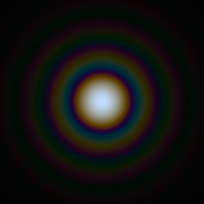
Artist: SiriusB
White-light imaging introduces another layer: chromatic aberration. Lenses have focal lengths that vary with wavelength unless corrected. Objective families differ in the degree of chromatic correction:
- Achromats bring two wavelengths into common focus and partially correct lateral color.
- Fluorite (semi-apochromat) objectives improve color correction and spherical aberration performance, often with higher NA options.
- Apochromats bring three or more wavelengths into common focus and correct lateral and axial color more thoroughly, supporting both high NA and excellent color fidelity.
Chromatic performance matters even for monochrome cameras because chromatic aberration affects how different spectral components of broadband illumination contribute to the image. If the microscope is used with discrete spectral bands (e.g., filtered illumination in transmission or fluorescence), matching the objective’s correction to the bandwidth in use can improve focus consistency and resolution across channels.
If you work primarily at a single wavelength band, optimizing for that band—in illumination and detection—can reduce chromatic issues. If you require accurate color rendering (for educational or documentation purposes), higher correction objectives and careful white balance become important to perceive specimen detail without color fringing.
Quantifying Resolution: Abbe, Rayleigh, Sparrow, and MTF
Resolution criteria encapsulate how close two features can be while still being distinctly recognized as separate. Different criteria reflect different definitions of “just resolved” based on diffraction theory and human perception. In microscopy, several are commonly referenced:
- Abbe’s Criterion: Historically introduced for periodic structures, emphasizing that at least the zeroth and first diffraction orders must be transmitted to form a resolvable image of a grating. In coherent illumination, the condenser and objective NA both appear in the limit; in incoherent brightfield, the practical cutoff is often discussed in terms of the objective’s NA and wavelength, aligning with the Rayleigh-style estimate.
- Rayleigh Criterion: Based on the first minimum of one Airy pattern coinciding with the central maximum of another, giving
d_R ≈ 0.61 λ / NAfor lateral resolution in incoherent imaging. This is widely used as a practical reference point. - Sparrow Criterion: Defines resolution at the point where the dip between two peaks vanishes; it yields a slightly smaller separation than Rayleigh, reflecting a different perceptual threshold.

Artist: Bautsch
Understanding MTF clarifies why simply meeting a theoretical “resolution limit” does not guarantee that the finest details are easily visible: as you approach the cutoff frequency, contrast becomes very low. That is why illumination geometry, condenser aperture, and stray light control (see Köhler illumination) are so important: they influence how much useful contrast the system preserves in the mid-to-high spatial frequency range where your finest specimen features lie.
In practice, resolution is often reported alongside contrast and signal-to-noise considerations. For instance, if the camera or display pipeline reduces dynamic range or adds noise, low-contrast fine details might be buried even if, in principle, the optics transmit them. Optimizing the entire chain—illumination, NA, aberration control, magnification, and sampling—ensures that theoretical limits are approached in real images.
Calibrating Field of View and Avoiding Empty Magnification
Empty magnification occurs when you increase image scale without adding real optical detail. Avoiding it requires connecting objective NA, magnification, and camera pixel size.
Two practical tools help:
- Field number and eyepiece scaling (for visual observation): The field number (FN) of an eyepiece, divided by objective magnification, approximates the field diameter at the specimen. For example,
field_diameter ≈ FN / M_objective. This is independent of NA but sets expectations about how much area you see. - Pixel size and total magnification (for cameras): Effective pixel size at the specimen is
p_sample = p_cam / M_total. This allows you to check Nyquist sampling relative to the Rayleigh estimated_R ≈ 0.61 λ / NA.
Example (purely illustrative): suppose a camera with 3.45 µm pixels is coupled to a 40× objective. If the total magnification onto the sensor is 40× (e.g., a 1× camera port), then p_sample = 3.45 µm / 40 = 0.086 µm/pixel. With green light (say, 550 nm) and NA = 0.75, the Rayleigh estimate is d_R ≈ 0.61 × 0.55 µm / 0.75 ≈ 0.447 µm. The Nyquist condition recommends p_sample ≤ 0.5 × d_R ≈ 0.224 µm. Since 0.086 µm < 0.224 µm, this configuration oversamples, which is acceptable. If we had a lower magnification or larger pixels resulting in p_sample > 0.224 µm, we would be undersampling and potentially losing high-frequency detail.
Lessons from this calculation:
- Sampling adequacy depends on both NA and magnification; low NA reduces the optical cutoff so fewer pixels are needed per millimeter of the specimen to achieve Nyquist sampling.
- Oversampling is common with high-magnification objectives and modern small-pixel sensors. It trades field of view and some per-pixel SNR but preserves detail. Binning or downsampling after acquisition can improve SNR while keeping spatial fidelity.
- Undersampling risks aliasing and lost detail. If you identify undersampling, consider increasing magnification (e.g., adding a relay lens), choosing a smaller-pixel camera, or using a higher-NA objective if specimen and illumination allow.
Finally, remember that magnification without NA is hollow. To resolve finer structures, increasing NA (through objective choice and appropriate immersion media) is the fundamental lever, supported by Köhler illumination and good sampling.
Frequently Asked Questions
Is higher numerical aperture always better?
Higher NA improves theoretical lateral and axial resolution by capturing higher-angle diffracted light. However, it comes with trade-offs: reduced depth of field, often shorter working distance, greater sensitivity to refractive index mismatch and cover glass thickness, and more demanding illumination conditions. In brightfield, you may also need to open the condenser aperture to match the objective NA; this can lower contrast for weakly scattering or absorbing specimens. Choose NA that matches your sample thickness, desired field of view, contrast needs, and mechanical constraints. For very thick or uneven specimens, a moderate NA can produce images that are easier to interpret, even if the ultimate resolution is lower.
How does Köhler illumination improve resolution and contrast?
Köhler illumination separates the source structure from the image-forming path by focusing the source at the condenser aperture plane and the field diaphragm at the specimen. This yields uniform illumination and independent controls for the illuminated area (field diaphragm) and the illumination NA (aperture diaphragm). When the aperture diaphragm is adjusted to provide sufficient condenser NA, high spatial frequencies in the specimen are excited, supporting the objective’s resolving power. At the same time, limiting the illuminated area with the field diaphragm reduces stray light, improving contrast and SNR. In short, Köhler ensures that the optical system’s theoretical resolution (set by NA and wavelength) is not squandered by uneven lighting or glare.
Wavelength Choice, Color, and Chromatic Effects
Resolution depends on wavelength: shorter wavelengths resolve finer detail. For the same NA, blue or near-UV illumination yields higher theoretical resolution than red illumination because the diffraction-limited spot size scales with λ. However, changing wavelength also changes sample absorption and scattering behavior and can influence photophysical responses. From a purely optical standpoint, the trend is straightforward: decreasing wavelength improves the achievable resolution given the same NA.
White-light imaging introduces another layer: chromatic aberration. Lenses have focal lengths that vary with wavelength unless corrected. Objective families differ in the degree of chromatic correction:
- Achromats bring two wavelengths into common focus and partially correct lateral color.
- Fluorite (semi-apochromat) objectives improve color correction and spherical aberration performance, often with higher NA options.
- Apochromats bring three or more wavelengths into common focus and correct lateral and axial color more thoroughly, supporting both high NA and excellent color fidelity.
Chromatic performance matters even for monochrome cameras because chromatic aberration affects how different spectral components of broadband illumination contribute to the image. If the microscope is used with discrete spectral bands (e.g., filtered illumination in transmission or fluorescence), matching the objective’s correction to the bandwidth in use can improve focus consistency and resolution across channels.
If you work primarily at a single wavelength band, optimizing for that band—in illumination and detection—can reduce chromatic issues. If you require accurate color rendering (for educational or documentation purposes), higher correction objectives and careful white balance become important to perceive specimen detail without color fringing.
Quantifying Resolution: Abbe, Rayleigh, Sparrow, and MTF
Resolution criteria encapsulate how close two features can be while still being distinctly recognized as separate. Different criteria reflect different definitions of “just resolved” based on diffraction theory and human perception. In microscopy, several are commonly referenced:
- Abbe’s Criterion: Historically introduced for periodic structures, emphasizing that at least the zeroth and first diffraction orders must be transmitted to form a resolvable image of a grating. In coherent illumination, the condenser and objective NA both appear in the limit; in incoherent brightfield, the practical cutoff is often discussed in terms of the objective’s NA and wavelength, aligning with the Rayleigh-style estimate.
- Rayleigh Criterion: Based on the first minimum of one Airy pattern coinciding with the central maximum of another, giving
d_R ≈ 0.61 λ / NAfor lateral resolution in incoherent imaging. This is widely used as a practical reference point. - Sparrow Criterion: Defines resolution at the point where the dip between two peaks vanishes; it yields a slightly smaller separation than Rayleigh, reflecting a different perceptual threshold.
While these points provide reference separations, a more complete way to quantify image-forming capability is through the Modulation Transfer Function (MTF). The MTF is the magnitude of the optical transfer function and describes how contrast at different spatial frequencies is transferred from object to image:
- Low spatial frequencies (broad features) are typically transferred with high contrast.
- High spatial frequencies (fine features) are transferred with lower contrast, approaching zero at the system cutoff.
Understanding MTF clarifies why simply meeting a theoretical “resolution limit” does not guarantee that the finest details are easily visible: as you approach the cutoff frequency, contrast becomes very low. That is why illumination geometry, condenser aperture, and stray light control (see Köhler illumination) are so important: they influence how much useful contrast the system preserves in the mid-to-high spatial frequency range where your finest specimen features lie.
In practice, resolution is often reported alongside contrast and signal-to-noise considerations. For instance, if the camera or display pipeline reduces dynamic range or adds noise, low-contrast fine details might be buried even if, in principle, the optics transmit them. Optimizing the entire chain—illumination, NA, aberration control, magnification, and sampling—ensures that theoretical limits are approached in real images.
Calibrating Field of View and Avoiding Empty Magnification
Empty magnification occurs when you increase image scale without adding real optical detail. Avoiding it requires connecting objective NA, magnification, and camera pixel size.
Two practical tools help:
- Field number and eyepiece scaling (for visual observation): The field number (FN) of an eyepiece, divided by objective magnification, approximates the field diameter at the specimen. For example,
field_diameter ≈ FN / M_objective. This is independent of NA but sets expectations about how much area you see. - Pixel size and total magnification (for cameras): Effective pixel size at the specimen is
p_sample = p_cam / M_total. This allows you to check Nyquist sampling relative to the Rayleigh estimated_R ≈ 0.61 λ / NA.
Example (purely illustrative): suppose a camera with 3.45 µm pixels is coupled to a 40× objective. If the total magnification onto the sensor is 40× (e.g., a 1× camera port), then p_sample = 3.45 µm / 40 = 0.086 µm/pixel. With green light (say, 550 nm) and NA = 0.75, the Rayleigh estimate is d_R ≈ 0.61 × 0.55 µm / 0.75 ≈ 0.447 µm. The Nyquist condition recommends p_sample ≤ 0.5 × d_R ≈ 0.224 µm. Since 0.086 µm < 0.224 µm, this configuration oversamples, which is acceptable. If we had a lower magnification or larger pixels resulting in p_sample > 0.224 µm, we would be undersampling and potentially losing high-frequency detail.
Lessons from this calculation:
- Sampling adequacy depends on both NA and magnification; low NA reduces the optical cutoff so fewer pixels are needed per millimeter of the specimen to achieve Nyquist sampling.
- Oversampling is common with high-magnification objectives and modern small-pixel sensors. It trades field of view and some per-pixel SNR but preserves detail. Binning or downsampling after acquisition can improve SNR while keeping spatial fidelity.
- Undersampling risks aliasing and lost detail. If you identify undersampling, consider increasing magnification (e.g., adding a relay lens), choosing a smaller-pixel camera, or using a higher-NA objective if specimen and illumination allow.
Finally, remember that magnification without NA is hollow. To resolve finer structures, increasing NA (through objective choice and appropriate immersion media) is the fundamental lever, supported by Köhler illumination and good sampling.
Frequently Asked Questions
Is higher numerical aperture always better?
Higher NA improves theoretical lateral and axial resolution by capturing higher-angle diffracted light. However, it comes with trade-offs: reduced depth of field, often shorter working distance, greater sensitivity to refractive index mismatch and cover glass thickness, and more demanding illumination conditions. In brightfield, you may also need to open the condenser aperture to match the objective NA; this can lower contrast for weakly scattering or absorbing specimens. Choose NA that matches your sample thickness, desired field of view, contrast needs, and mechanical constraints. For very thick or uneven specimens, a moderate NA can produce images that are easier to interpret, even if the ultimate resolution is lower.
What pixel size should my camera have for a given objective?
Use the Nyquist guideline. Compute the sample-plane pixel size p_sample = p_cam / M_total and compare it to half the Rayleigh estimate 0.5 × (0.61 λ / NA). If p_sample is smaller than this value, you are sampling adequately (or even oversampling). If it is larger, you risk undersampling. For example, with green light and NA around 0.75, half the Rayleigh-limited distance is roughly a few tenths of a micrometer. Align your magnification and pixel size so that p_sample is below that threshold. If not, consider increasing magnification onto the sensor, selecting a smaller-pixel camera, or using a higher-NA objective if the specimen and illumination permit.
Final Thoughts on Choosing the Right Numerical Aperture and Illumination Strategy
Microscopy image quality hinges on a coherent chain of decisions: numerical aperture sets the theoretical resolving power; Köhler illumination and condenser aperture determine how that power translates into usable contrast; magnification and sampling decide whether your camera records the available detail without aliasing; and aberration control via correct immersion media and cover glass practices preserves performance in real specimens.
Key takeaways:
- NA and wavelength define the resolution ceiling: lateral detail scales as
∼0.61 λ / NA. - Köhler illumination provides uniform lighting and decouples field and aperture control, essential for predictable contrast and efficient high-NA imaging.
- Condenser NA should be set near the objective NA for brightfield resolution; adjust modestly to balance contrast and DOF.
- Sampling must satisfy Nyquist: target at least two pixels per smallest resolvable feature to avoid aliasing; slight oversampling is generally beneficial.
- Immersion and aberration control ensure that labeled NA translates to real-world performance, especially at high NA.
If you’re planning your next observation session or upgrading a component, start by articulating your imaging goal (finest detail, contrast visibility, or field coverage), then choose NA, illumination, and sampling accordingly. To dive deeper into related fundamentals and practical checklists in future issues, consider subscribing to our newsletter—stay up to date as we explore more microscopy principles and hands-on guidance.

