Numerical Aperture, Resolution, and Real Magnification
Table of Contents
- What Is Numerical Aperture (NA) and Why It Matters
- Magnification vs. Resolution: Avoiding Empty Magnification
- Abbe and Rayleigh Resolution Criteria Explained
- Wavelength, Refractive Index, and Immersion Media
- Contrast, Point Spread Function, and MTF Basics
- Depth of Field vs. Depth of Focus in Microscopy
- Sampling, Pixel Size, and the Nyquist Criterion
- Choosing Objectives: NA, Working Distance, and Field
- Common Mistakes and How to Fix Soft Images
- Frequently Asked Questions
- Final Thoughts on Choosing the Right NA and Magnification
What Is Numerical Aperture (NA) and Why It Matters
In optical microscopy, numerical aperture (NA) is the single most important specification for image sharpness and resolving fine detail. While magnification tells you how large a specimen appears, NA determines how much angular range of light the objective lens can accept from the sample. The greater that angular range, the finer the details that can be captured.
By definition, numerical aperture is
NA = n · sin(θ)

Attribution: PaulT (Gunther Tschuch)
where n is the refractive index of the medium between the front lens and the specimen (air ≈ 1.0, water ≈ 1.33, standard immersion oil ≈ 1.515), and θ is the half-angle of the maximum cone of light that can enter or exit the objective. Because sin(θ) cannot exceed 1, the only way to push NA high is to increase n (using immersion media) and design objectives with large acceptance angles.
High NA has sweeping consequences:
- Higher lateral resolution: Smaller features can be separated, as detailed in Abbe and Rayleigh Resolution Criteria.
- Greater light-gathering power: For incoherent imaging, detected signal scales strongly with NA; high NA improves signal and contrast for fine structures.
- Shallower depth of field: As NA increases, the in-focus axial range shrinks dramatically (see Depth of Field vs. Depth of Focus).
- Sensitivity to alignment and coverslip conditions: High-NA optics are more sensitive to refractive index mismatch and coverslip thickness errors (discussed in Wavelength, Refractive Index, and Immersion Media).
In short, if you want a sharper image or to resolve smaller features, you usually need to increase NA, not just magnification. This distinction is central to avoiding empty magnification, a topic we expand on next.
Magnification vs. Resolution: Avoiding Empty Magnification
Magnification enlarges an image; resolution determines how much detail it contains. You can enlarge a blurred image, but you can’t invent detail that the optics never captured. Empty magnification occurs when the total magnification is increased beyond what the objective’s NA and the wavelength of light can support. The result is a bigger picture of the same blur.
Three practical guidelines help avoid empty magnification:
- Match magnification to NA and wavelength: The smallest resolvable lateral detail for widefield imaging is on the order of ~0.5–0.6 λ/NA depending on the criterion used. If your pixels at the specimen are much larger than this, you are undersampling; if they are much smaller, you are likely oversampling (see Sampling, Pixel Size, and the Nyquist Criterion).
- Avoid chasing total magnification numbers: For eyepiece viewing, a traditional rule-of-thumb is to keep total magnification roughly between 500× NA and 1000× NA for useful visual observation. This range is indicative rather than strict and depends on the viewer’s acuity and illumination quality.
- For cameras, size the image to the pixels: Choose objective and intermediate magnification such that the effective pixel size at the specimen meets Nyquist sampling for your objective/illumination wavelength. This is more precise than a total magnification rule (see Sampling).
When you balance magnification against resolution, you get images that are both sharp and information-rich. Overmagnification wastes light and frame rate, while undermagnification throws away real detail the optics are already delivering.
Abbe and Rayleigh Resolution Criteria Explained
Two related but distinct ways to quantify resolution in optical microscopy are widely cited: Abbe’s diffraction limit and the Rayleigh criterion. Both arise from the wave nature of light and the diffraction of the objective pupil.
Lateral (XY) resolution
- Abbe limit for periodic structures: For incoherent illumination imaging a periodic structure, the smallest resolvable period has a spacing roughly given by
d ≈ λ / (2 NA). This criterion is tied to whether the necessary diffraction orders pass through the objective aperture and reach the image plane. - Rayleigh criterion for point-like features: For two point sources, the Rayleigh criterion defines them as just resolvable when the first minimum of one diffraction pattern (Airy disk) coincides with the central maximum of the other. In the specimen plane, a commonly used expression is
d ≈ 0.61 λ / NAfor incoherent imaging.
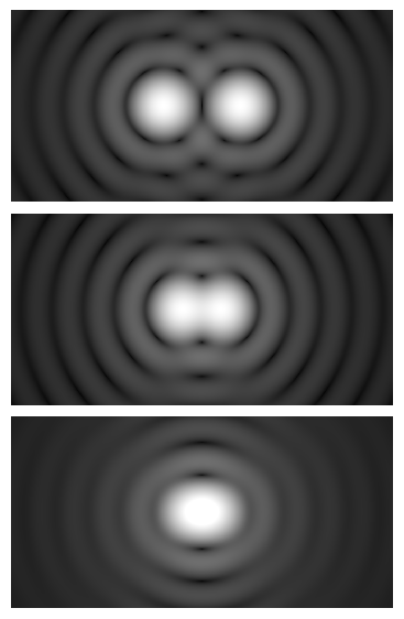
This image uses a nonlinear color scale (specifically, the fourth root) in order to better show the minima and maxima.
Attribution: Spencer Bliven
These expressions differ by a numerical factor (0.5 vs. 0.61) because they formalize different resolution tests—periodic structures versus isolated point-like features. They both show the same scaling: resolution improves (smaller d) with shorter wavelength and higher NA.
Axial (Z) resolution
Axial resolution is the system’s ability to distinguish features separated along the optical axis. Approximations (for widefield, incoherent illumination) often take the form:
Δz ≈ (2 n λ) / NA²
Here, n is the refractive index of the immersion medium. The main takeaway is that axial resolution scales with 1/NA², so doubling NA can improve axial resolution by roughly a factor of four—all else equal.
Implications and limits
- For widefield brightfield/fluorescence, these limits describe what the objective can do under ideal alignment and good illumination (see PSF and MTF Basics).
- Techniques like confocal and structured illumination microscopy (SIM) can improve contrast and, in certain cases, effective resolution compared with widefield, but they rely on different detection or illumination strategies beyond the scope of this fundamentals article.
- In practice, sample properties (scattering, thickness, refractive mismatch) and system alignment can keep you from ever reaching the theoretical diffraction limit.
Wavelength, Refractive Index, and Immersion Media
Resolution depends on λ (wavelength) and NA. We typically quote resolution using a wavelength representative of the illumination spectrum or the emission band for fluorescence. Shorter wavelengths provide higher resolution; for example, blue light resolves finer detail than red light with the same objective and medium.
Refractive index and NA
Because NA = n · sin(θ), increasing the refractive index of the medium in front of the objective increases NA. That is why immersion objectives exist:

Attribution: Thebiologyprimer
- Air objectives (n ≈ 1.0): Typically NA up to ~0.95 in practical designs.
- Water immersion (n ≈ 1.33): Common in live-cell imaging where water-like refractive index improves mismatch performance in aqueous samples.
- Oil immersion (n ≈ 1.515): Enables very high NA (≥ 1.4 in many designs), offering superior lateral and axial resolution with appropriate samples and coverslips.
- Glycerol and silicone oil immersion: Intermediate indices that can reduce mismatch in thick, cleared, or living tissues while offering high NA options.
Coverslip thickness and correction collars
High-NA objectives assume a specific coverslip thickness (often 0.17 mm for No. 1.5H coverslips) and refractive properties. Deviation from this target introduces spherical aberration that broadens the point spread function (PSF) and reduces contrast. Objectives with a correction collar allow you to adjust for small thickness variations by compensating internal lens spacing. If your objective has a collar, use it carefully for best performance, especially at NA ≥ 0.8.
Refractive index mismatch and spherical aberration
Imaging into thick specimens with refractive indices that do not match the immersion medium (e.g., water sample with oil immersion lens) can cause depth-dependent aberrations. Symptoms include loss of contrast, axial elongation of features, and a systematic decrease in resolution with depth. Choosing an immersion medium and objective designed for your specimen’s refractive index profile can improve results dramatically (see Choosing Objectives).
Contrast, Point Spread Function, and MTF Basics
Resolution tells you the smallest structure you could theoretically separate; contrast and the point spread function (PSF) describe how sharply details appear. Even at the diffraction limit, the image of a point is not a point. It is a central bright spot (the Airy disk) surrounded by rings whose intensity decays with radius. The PSF encodes this intensity distribution.

Attribution: Anaqreon
From PSF to contrast
When you image, the sample’s structure is convolved with the PSF. If the PSF is broad (from low NA or aberrations), fine features blur together, and contrast at high spatial frequencies drops. If the PSF is tight (high NA, well-corrected optics), more of the fine structure survives to the image.
Modulation Transfer Function (MTF)
The MTF is the magnitude of the optical transfer function (OTF), which is the Fourier transform of the PSF. It tells you how much contrast at each spatial frequency the optical system preserves. Two key facts guide practical decisions:
- Cutoff frequency for incoherent imaging: There is a highest spatial frequency the system can transfer. For widefield, incoherent imaging, this cutoff is approximately
f_c ≈ 2 NA / λ. Frequencies higher than this do not pass through the optics. - Contrast rolls off before cutoff: Even before the cutoff, contrast progressively falls, so small features may be technically resolvable but appear with low contrast unless illumination and detection SNR are high (see Sampling and SNR).
Because MTF falls with spatial frequency, the mere act of magnifying an image won’t recover contrast of lost frequencies. That’s why empty magnification does not help; it spreads existing information over more pixels without adding new detail.
Depth of Field vs. Depth of Focus in Microscopy
Depth of field (DOF) is the axial range in the specimen over which features appear acceptably sharp. Depth of focus is the corresponding tolerance in the image plane around the sensor or eyepiece where the image remains in focus. These are related but not the same; one lives in object space, the other in image space.
How NA affects DOF
In diffraction-limited microscopy, DOF decreases approximately with 1/NA². As NA increases, the cone of focused light becomes steeper, reducing the axial range over which features remain sharp. Very high NA objectives produce thin optical sections, beneficial for isolating planes in thick samples but challenging for focusing and mechanical stability.
Wavelength and coherence
Shorter wavelengths produce smaller PSFs and thus thinner DOF, all else equal. Illumination coherence also affects exact DOF expressions. For practical widefield setups using Köhler illumination, the common trend remains: higher NA and shorter λ produce shallower DOF.
Depth of focus on the camera side
Depth of focus—the tolerance at the sensor—grows with magnification and wavelength, and decreases with NA. A higher objective magnification spreads the PSF over more sensor pixels, making the captured image somewhat more tolerant of small sensor-plane defocus. This does not change the true object-side DOF, but it can influence how sensitive your camera focus is to minute movements of the stage or tube lens.
Operationally, if you find focusing difficult or drift intolerable, revisit objective choice (NA, working distance) and improve alignment and illumination. Note that techniques such as focus stacking create an extended-DOF composite but do not increase the intrinsic optical DOF.
Sampling, Pixel Size, and the Nyquist Criterion
If NA and wavelength define what detail the optics can transmit, sampling defines what detail your camera can actually record. The Nyquist sampling theorem states that to capture frequencies up to a maximum frequency f_max, you must sample at least at f_s ≥ 2 · f_max. In microscopy, f_max is limited by the optics’ cutoff frequency and by practical contrast fall-off.
Relating pixel size to specimen scale
The effective pixel size at the specimen is
p_spec = p_sensor / M_total
where p_sensor is the pixel pitch on the camera sensor and M_total is the total magnification between the specimen and the sensor (objective magnification times any intermediate optics).
How fine should sampling be?
- Using the Rayleigh criterion as a characteristic feature size (
d_R ≈ 0.61 λ / NA), a common practical guideline is to sample withp_spec ≤ d_R / 2, i.e., ~0.3 λ/NA. - Using the OTF cutoff for incoherent imaging (
f_c ≈ 2 NA / λ), strict Nyquist for the highest transferable frequency yieldsp_spec ≤ 1 / (2 f_c) = λ / (4 NA), i.e., ~0.25 λ/NA.
Either way, a practical target is often p_spec between ~0.25 and 0.33 λ/NA. Sampling much finer than this (e.g., p_spec ≪ 0.25 λ/NA) usually does not reveal more optical detail but increases data size and may lower SNR per pixel; sampling much coarser risks aliasing and loss of resolvable information.
Worked example
Suppose you are imaging with a green emission at λ = 550 nm and an objective with NA = 1.3. A target p_spec using the OTF-based bound is:
p_spec ≤ λ / (4 NA) = 550 nm / (4 × 1.3) ≈ 106 nm
If your camera has 6.5 μm pixels, the required total magnification to reach ~106 nm at the specimen is:
M_total ≥ p_sensor / p_spec = 6.5 μm / 0.106 μm ≈ 61×
With a 60× objective and 1× tube lens, you’re essentially at Nyquist by this conservative criterion. If you used the Rayleigh-based ~0.3 λ/NA target, the required magnification would be somewhat lower. This illustrates how magnification choices flow directly from NA, λ, and pixel size.
Simple calculator snippet
Below is a small pseudocode/Python-like snippet to estimate recommended magnification for widefield, incoherent imaging. It uses the OTF-based Nyquist target by default and also prints a Rayleigh-based target.
# Inputs: wavelength (lambda_nm), NA, pixel size (p_sensor_um)
# Outputs: recommended total magnification for two sampling targets


def recommended_mag(lambda_nm, NA, p_sensor_um):
    # Convert nm to um
    lam_um = lambda_nm / 1000.0
    # Specimen pixel size targets
    p_spec_otf = lam_um / (4.0 * NA)        # ~0.25 λ/NA
    p_spec_ray = 0.61 * lam_um / (2.0 * NA) # ~0.305 λ/NA
    # Required total magnification
    M_otf = p_sensor_um / p_spec_otf
    M_ray = p_sensor_um / p_spec_ray
    return M_otf, M_ray

# Example: λ = 550 nm, NA = 1.3, pixel = 6.5 μm
M_otf, M_ray = recommended_mag(550, 1.3, 6.5)
print(f"Nyquist (OTF cutoff) target M ≈ {M_otf:.1f}×")
print(f"Rayleigh-based target M ≈ {M_ray:.1f}×")
Use this as a guide rather than a strict standard. Actual needs depend on your sample’s contrast at high spatial frequencies and your signal-to-noise constraints.
Choosing Objectives: NA, Working Distance, and Field
Selecting an objective lens is a multi-parameter trade-off. Beyond nominal magnification, consider NA, immersion medium, working distance, field flatness, and correction level. The right choice depends on your sample and your detection method (human eye through eyepieces vs. camera).
NA and magnification

Attribution: QuodScripsiScripsi
- Prioritize NA for detail: For two objectives of equal magnification, the one with higher NA generally offers better resolution and light collection.
- Beware of low-NA, high-magnification combinations: For example, a 100× objective with NA 0.8 will not resolve as much as a 60× objective with NA 1.4. Do not equate magnification with detail.
Working distance (WD)
Working distance is the clearance between the front lens and the specimen when in focus. High NA typically implies shorter WD, although specialized long-WD objectives exist. Consider WD when:
- Your specimens are thick or uneven.
- You need to use micro-manipulators or probes near the focal plane.
- There is a risk of contacting the sample with the front lens, especially with oil immersion objectives.
Field of view (FOV) and field number (FN)
For eyepiece viewing, the field number (FN, in mm) of the eyepiece determines the diameter of the intermediate image visible. The specimen-space field diameter is approximately:
FOV_spec ≈ FN / M_obj
For camera imaging, the FOV is set by the sensor dimensions divided by total magnification. If you need to cover a larger area at a given NA, consider stitching multiple images or exploring lower magnification objectives with comparably high NA (rare but valuable).
Chromatic and flatness corrections
Objectives differ in their correction level for chromatic focus shift, lateral color, and field curvature. For critical imaging across color channels (fluorescence or RGB brightfield), higher correction classes can maintain focus and magnification consistency across wavelengths. Flat-field (plan) objectives keep the field sharp toward the edges—important for large sensors or quantitative imaging.
Immersion and sample compatibility
Choose immersion media to match your sample’s environment and depth. For live, aqueous samples or thick tissue where refractive mismatch degrades performance, water-immersion or silicone oil objectives may yield tighter PSFs deeper into the specimen than standard oil immersion, even at slightly lower NA. See Wavelength, Refractive Index, and Immersion Media for considerations.
Common Mistakes and How to Fix Soft Images
Soft, low-contrast images often come from correctable issues rather than inherent diffraction limits. Before upgrading hardware, check the following.
1) Mistaking magnification for resolution
Symptom: Big images with no added detail. Fix: Increase NA (appropriate immersion, higher-NA objective) or adjust sampling to match the existing NA. See Magnification vs. Resolution.
2) Undersampling (aliasing)
Symptom: Moiré patterns or loss of fine textures. Fix: Increase total magnification to reduce p_spec, or use a camera with smaller pixels. Review Sampling and Pixel Size.
3) Oversampling (needlessly small pixels)
Symptom: Large files with no gain in detail, lower SNR per pixel. Fix: Reduce total magnification or bin pixels to boost SNR and frame rate, while staying within Nyquist.
4) Refractive index mismatch
Symptom: Features blur and elongate with depth. Fix: Use the immersion medium and objective designed for your sample’s refractive index; consider water or silicone immersion for aqueous or thick specimens (see Immersion Media).
5) Coverslip thickness errors
Symptom: High-NA air objectives underperform, or oil objectives show low contrast. Fix: Use specified coverslips (often No. 1.5H, ~0.17 mm), and adjust the correction collar if available.
6) Illumination alignment
Symptom: Uneven or low-contrast brightfield images. Fix: Align Köhler illumination to provide even, controllable illumination NA. Suboptimal illumination reduces contrast at useful spatial frequencies.
7) Contamination or damage on optics
Symptom: Haze or flare, especially in brightfield. Fix: Inspect and carefully clean objective front elements and coverslips following manufacturer-safe methods. Avoid scratching high-NA front lenses.
8) Mechanical instability
Symptom: Images sharpen and blur with tiny touches; z-stacks misregister. Fix: Improve focusing mechanics, check stage backlash, and ensure secure mounting. Pair these improvements with appropriate DOF expectations from Depth of Field.
Frequently Asked Questions
Is it better to use a 100× objective than a 60× objective for more detail?
Not automatically. What matters most is the NA and optical quality. A 60× objective with NA 1.40 can resolve finer detail than a 100× objective with NA 0.90. Choose based on NA, immersion medium suitability, and your sampling setup, not magnification alone. If your camera pixel size already satisfies Nyquist with a 60×/1.4, moving to 100× may offer little benefit and could reduce field of view and light efficiency.
How do I pick the right camera pixel size for my objectives?
Work backward from the optics. Decide the wavelength band of interest and the objective NA. Target a specimen pixel size around 0.25–0.33 λ/NA for widefield, incoherent imaging. Then choose magnification (objective × intermediates) so that p_spec = p_sensor / M_total meets that target. If your camera pixels are large, you may need more magnification; if they are small, you can often use less magnification and gain field of view and sensitivity without losing detail.
Final Thoughts on Choosing the Right NA and Magnification
The path to sharper, more informative micrographs starts with understanding how NA, wavelength, and sampling interact. Objectives with higher NA—and immersion media that support them—set the fundamental limit on what details you can resolve. Magnification then scales that optical information to your eye or sensor; used wisely, it preserves detail and contrast without wasting light or storage.

Attribution: Ernst Leitz (Firm)
As you refine your setup, revisit these checkpoints:
- Let NA guide you when detail matters.
- Ground magnification choices in Nyquist sampling and your camera’s pixel size.
- Pay attention to immersion, refractive index, and coverslip to keep the PSF tight.
- Use contrast and MTF thinking to set realistic expectations for small, low-contrast features.
With these fundamentals in hand, you can assess trade-offs with confidence, make better objective and camera pairings, and capture images that reveal what your specimens truly contain. If you enjoyed this deep dive into microscope fundamentals, explore our other articles, and subscribe to the newsletter for future installments on optics, imaging theory, and practical microscopy tips.

